3MC Course on Epidemiological Modelling
Course material (slides and code).
View the Project on GitHub julien-arino/3MC-course-epidemiological-modelling
Lecture 05 - Metapopulation epidemic models
5 April 2022
Julien Arino ![]()
![]()
![]()
Department of Mathematics & Data Science Nexus University of Manitoba*
Canadian Centre for Disease Modelling Canadian COVID-19 Mathematical Modelling Task Force NSERC-PHAC EID Modelling Consortium (CANMOD, MfPH, OMNI/RÉUNIS)
Outline
- Formulating metapopulation models
- Basic mathematical analysis
- $\mathcal{R}_0$ is not the panacea - An urban centre and satellite cities
- Problems specific to metapopulations
- Global stability considerations
Formulating metapopulation models
General principles (1)
-
$ \mathcal{P} $ geographical locations (patches) in a set $\mathcal{P}$ (city, region, country..) - Patches are vertices in a graph
- Each patch $p\in\mathcal{P}$ contains compartments $\mathcal{C}_p\subseteq\mathcal{C}$
- individuals susceptible to the disease
- individuals infected by the disease
- different species affected by the disease
- etc.
- individuals susceptible to the disease

General principles (2)
- Compartments may move between patches, with $m_{cqp}$ rate of movement of individuals from compartment $c\in\mathcal{C}$ from patch $p\in\mathcal{P}$ to patch $q\in\mathcal{P}\setminus{p}$
- Movement instantaneous and no death during movement
- $\forall c\in\mathcal{C}$, defines a digraph $\mathcal{G}^c$ with arcs $\mathcal{A}^c$
- Arc from $p$ to $q$ if $m_{cqp}>0$, absent otherwise
-
$ \mathcal{C} $ compartments, so each $(p,q)$ can have at most $ \mathcal{C} $ arrows $\rightarrow$ multi-digraph
The underlying mobility model
$N_{cp}$ population of compartment $c\in\mathcal{C}$ in patch $p\in\mathcal{P}$
Assume no birth or death. Balance inflow and outflow
\(\begin{align} N_{cp}' &= \left(\sum_{q\in\mathcal{P}\setminus\{p\}} m_{cpq}N_{cq}\right)-\left(\sum_{q\in\mathcal{P}\setminus\{p\}} m_{cqp}\right)N_{cp} \\ &\\ \text{or} & \\ &\\ N_{cp}' &= \sum_{q\in\mathcal{P}} m_{cpq}N_{cq} \qquad \tag{1}\label{eq:dNcp} \end{align}\) when we write \(m_{cpp}=-\sum_{q\in\mathcal{P}\setminus\{p\}} m_{cqp}\)
The toy SLIRS model in patches

$B(N)$ is the birth rate (typically $b$ or $bN$)
$L$ = latently infected ($\simeq E$ exposed, although the latter term is ambiguous)
$|\mathcal{P}|$-SLIRS model
\[\begin{align} S_{p}' &=\mathcal{B}_p\left(N_p\right)+\nu_pR_p-\Phi_p-d_pS_p \color{red}{+\textstyle{\sum_{q\in\mathcal{P}}} m_{Spq}S_{q}} \tag{2a}\label{sys:pSLIRS_dS} \\ L_{p}' &=\Phi_p-\left( \varepsilon_{p}+d_{p}\right)L_{p} \color{red}{+\textstyle{\sum_{q\in\mathcal{P}}} m_{Lpq}L_{q}} \tag{2b}\label{sys:pSLIRS_dL} \\ I_{p}' &=\varepsilon_pL_p-(\gamma_p+d_p)I_p \color{red}{+\textstyle{\sum_{q\in\mathcal{P}}} m_{Ipq}I_{q}} \tag{2c}\label{sys:pSLIRS_dI} \\ R_{p}' &=\gamma _{p}I_{p}-\left(\nu_{p}+d_{p}\right)R_{p} \color{red}{+\textstyle{\sum_{q\in\mathcal{P}}} m_{Rpq}R_{q}} \tag{2d}\label{sys:pSLIRS_dR} \end{align}\]with incidence \(\Phi_p=\beta_p\frac{S_pI_p}{N_p^{q_p}},\qquad q_p\in\{0,1\} \tag{2e}\label{sys:pSLIRS_incidence}\)
$|\mathcal{S}|\;|\mathcal{P}|$-SLIRS (multiple species)
$\mathcal{S}$ a set of species \(\begin{align} S_{sp}' &= \mathcal{B}_{sp}(N_{sp})+\nu_{sp}R_{sp}-\Phi_{sp}-d_{sp}S_{sp} \color{red}{+\textstyle{\sum_{q\in\mathcal{P}}} m_{Sspq}S_{sq}} \tag{3a}\label{sys:spSLIRS_dS} \\ L_{sp}' &= \Phi_{sp}-(\varepsilon_{sp}+d_{sp})L_{sp} \color{red}{+\textstyle{\sum_{q\in\mathcal{P}}}m_{Lspq}L_{sq}} \tag{3b}\label{sys:spSLIRS_dL} \\ I_{sp}' &= \varepsilon_{sp}L_{sp}-(\gamma_{sp}+d_{sp})I_{sp} \color{red}{+\textstyle{\sum_{q\in\mathcal{P}}} m_{Ispq}I_{sq}} \tag{3c}\label{sys:spSLIRS_dI} \\ R_{sp} &= \gamma _{sp}I_{sp}-(\nu_{sp}+d_{sp})R_{sp} \color{red}{+\textstyle{\sum_{q\in\mathcal{P}}} m_{Rspq}R_{sq}} \tag{3d}\label{sys:spSLIRS_dR} \end{align}\)
with incidence \(\Phi_{sp}=\sum_{k\in\mathcal{S}}\beta_{skp}\frac{S_{sp}I_{kp}}{N_p^{q_p}},\qquad q_p\in\{0,1\} \tag{3e}\label{sys:spSLIRS_incidence}\)
$|\mathcal{P}|^2$-SLIRS (residency patch/movers-stayers)
\[\begin{align} S_{pq}' =& \mathcal{B}_{pq}\left(N_p^r\right)+\nu_{pq} R_{pq}-\Phi_{pq}-d_{pq}S_{pq} \color{red}{+\textstyle{\sum_{k\in\mathcal{P}}} m_{Spqk}S_{pk}} \tag{4a}\label{sys:ppSLIRS_dS} \\ L_{pq}' =& \Phi_{pq} -(\varepsilon_{pq}+d_{pq})L_{pq} \color{red}{+\textstyle{\sum_{k\in\mathcal{P}}} m_{Lpqk}L_{pk}} \tag{4b}\label{sys:ppSLIRS_dL} \\ I_{pq}' =& \varepsilon_{pq} L_{pq} -(\gamma_{pq}+d_{pq})I_{pq} \color{red}{+\textstyle{\sum_{k\in\mathcal{P}}} m_{Ipqk}I_{pk}} \tag{4c}\label{sys:ppSLIRS_dI} \\ R_{pq}' =& \gamma_{pq} I_{pq} -(\nu_{pq}+d_{pq})R_{pq} \color{red}{+\textstyle{\sum_{k\in\mathcal{P}}} m_{Rpqk}R_{pk}} \tag{4d}\label{sys:ppSLIRS_dR} \end{align}\]with incidence \(\Phi_{pq}=\sum_{k\in\mathcal{P}}\beta_{pqk}\frac{S_{pq}I_{kq}}{N_p^{q_q}},\qquad q_q=\{0,1\} \tag{4e}\label{sys:ppSLIRS_incidence}\)
General metapopulation epidemic models
$\mathcal{U}\subsetneq\mathcal{C}$ uninfected and $\mathcal{I}\subsetneq\mathcal{C}$ infected compartments, $\mathcal{U}\cup\mathcal{I}=\mathcal{C}$ and $\mathcal{U}\cap\mathcal{I}=\emptyset$
For $k\in\mathcal{U}$, $\ell\in\mathcal{I}$ and $p\in\mathcal{P}$, \(\begin{align} s_{kp}' &= f_{kp}(S_p,I_p)+\sum_{q\in\mathcal{P}} m_{kpq}s_{kq} \tag{5a}\label{sys:general_metapop_ds} \\ i_{\ell p}' &= g_{\ell p}(S_p,I_p)+\sum_{q\in\mathcal{P}} m_{\ell pq}i_{\ell q} \tag{5b}\label{sys:general_metapop_di} \end{align}\) where $S_p=(s_{1p},\ldots,s_{|\mathcal{U}|p})$ and $I_p=(i_{1p},\ldots,i_{|\mathcal{I}|p})$
Basic mathematical analysis
Analysis - Toy system
For simplicity, consider $|\mathcal{P}|$-SLIRS with $\mathcal{B}_p(N_p)=\mathcal{B}_p$ \(\begin{align} S_{p}' &=\mathcal{B}_p-\Phi_p-d_pS_p+\nu_pR_p +\textstyle{\sum_{q\in\mathcal{P}}} m_{Spq}S_{q} \tag{6a}\label{sys:pSLIRS_toy_dS} \\ L_{p}' &=\Phi_p-\left( \varepsilon_{p}+d_{p}\right)L_{p} +\textstyle{\sum_{q\in\mathcal{P}}} m_{Lpq}L_{q} \tag{6b}\label{sys:pSLIRS_toy_dL} \\ I_{p}' &=\varepsilon_pL_p-(\gamma_p+d_p)I_p +\textstyle{\sum_{q\in\mathcal{P}}} m_{Ipq}I_{q} \tag{6c}\label{sys:pSLIRS_toy_dI} \\ R_{p}' &=\gamma _{p}I_{p}-\left(\nu_{p}+d_{p}\right)R_{p} +\textstyle{\sum_{q\in\mathcal{P}}} m_{Rpq}R_{q} \tag{6d}\label{sys:pSLIRS_toy_dR} \end{align}\)
with incidence \(\Phi_p=\beta_p\frac{S_pI_p}{N_p^{q_p}},\qquad q_p\in\{0,1\} \tag{6e}\label{sys:pSLIRS_toy_incidence}\)
| System of $4 | \mathcal{P} | $ equations |
Size is not that bad..
| System of $4 | \mathcal{P} | $ equations !!! |
However, a lot of structure:
-
$ \mathcal{P} $ copies of individual units, each comprising 4 equations - Dynamics of individual units well understood
- Coupling is linear
$\implies$ Good case of large-scale system (matrix analysis is your friend)
Notation in what follows
-
$M\in\mathcal{M}n(\mathbb{R})=\mathbb{R}^{n\times n}$ a square matrix with entries denoted $m{ij}$
-
$M\geq\mathbf{0}$ if $m_{ij}\geq 0$ for all $i,j$ (could be the zero matrix); $M>\mathbf{0}$ if $M\geq\mathbf{0}$ and $\exists i,j$ with $m_{ij}>0$; $M\gg\mathbf{0}$ if $m_{ij}>0$ $\forall i,j=1,\ldots,n$. Same notation for vectors
-
$\sigma(M)={\lambda\in\mathbf{C}; M\lambda=\lambda\mathbf{v}, \mathbf{v}\neq\mathbf{0}}$ spectrum of $M$
-
$\rho(M)=\max_{\lambda\in\sigma(M)}{ \lambda }$ spectral radius -
$s(M)=\max_{\lambda\in\sigma(M)}{\Re(\lambda)}$ spectral abscissa (or stability modulus)
- $M$ is an M-matrix if it is a Z-matrix ($m_{ij}\leq 0$ for $i\neq j$) and $M = s\mathbb{I}-A$, with $A\geq 0$ and $s\geq \rho(A)$
Behaviour of the total population
Consider behaviour of $N_p=S_p+L_p+I_p+R_p$. We have \(\begin{aligned} N_p' &=\mathcal{B}_p\cancel{-\Phi_p}-d_pS_p\cancel{+\nu_pR_p} +\textstyle{\sum_{q\in\mathcal{P}}} m_{Spq}S_{q} \\ &\quad \cancel{+\Phi_p}-\left(\cancel{\varepsilon_{p}} +d_{p}\right)L_{p} +\textstyle{\sum_{q\in\mathcal{P}}} m_{Lpq}L_{q} \\ &\quad \cancel{+\varepsilon_pL_p}-(\cancel{\gamma_p}+d_p)I_p +\textstyle{\sum_{q\in\mathcal{P}}} m_{Ipq}I_{q} \\ &\quad \cancel{+\gamma _{p}I_{p}} -\left(\cancel{\nu_{p}}+d_{p}\right)R_{p} +\textstyle{\sum_{q\in\mathcal{P}}} m_{Rpq}R_{q} \end{aligned}\)
So \(N_p'=\mathcal{B}_p-d_pN_p +\sum_{X\in\{S,L,I,R\}}\sum_{q\in\mathcal{P}} m_{Xpq}X_{q}\)
Vector / matrix form of the equation
We have \(N_p'=\mathcal{B}_p-d_pN_p +\sum_{X\in\{S,L,I,R\}}\sum_{q\in\mathcal{P}} m_{Xpq}X_{q}\) Write this in vector form \(\tag{7}\label{sys:pSLIRS_dN_general} \mathbf{N}'=\mathbf{b}-\mathbf{d}\mathbf{N}+\sum_{X\in\{S,L,I,R\}}\mathcal{M}^X\mathbf{X}\) where $\mathbf{b}=(\mathcal{B}1,\ldots,\mathcal{B}{|\mathcal{P}|})^T,\mathbf{N}=(N_1,\ldots,N_{|\mathcal{P}|})^T,\mathbf{X}=(X_1,\ldots,X_{|\mathcal{P}|})^T\in\mathbb{R}^{|\mathcal{P}|},$ $\mathbf{d},\mathcal{M}^X$ $|\mathcal{P}|\times|\mathcal{P}|$-matrices with \(\mathbf{d}=\mathsf{diag}\left(d_1,\ldots,d_{|\mathcal{P}|}\right)\)
The movement matrix
\[\mathcal{M}^c= \begin{pmatrix} -\sum_{q\in\mathcal{P}} m_{cq1} & m_{c12} & & m_{c1|\mathcal{P}|} \\ m_{c21} & -\sum_{q\in\mathcal{P}} m_{cq2} & & m_{c2|\mathcal{P}|} \\ & & & \\ m_{c|\mathcal{P}|1} & m_{c|\mathcal{P}|2} & & -\sum_{q\in\mathcal{P}} m_{cq|\mathcal{P}|} \end{pmatrix}\]The nice case
Recall that \(\tag{7} \mathbf{N}'=\mathbf{b}-\mathbf{d}\mathbf{N}+\sum_{X\in\{S,L,I,R\}}\mathcal{M}^X\mathbf{X}\)
Suppose movement rates equal for all compartments, i.e., \(\mathcal{M}^S=\mathcal{M}^L=\mathcal{M}^I=\mathcal{M}^R=:\mathcal{M}\) Then \(\begin{align} \mathbf{N}' &= \mathbf{b}-\mathbf{d}\mathbf{N}+\mathcal{M}\sum_{X\in\{S,L,I,R\}}\mathbf{X}\\ &= \mathbf{b}-\mathbf{d}\mathbf{N}+\mathcal{M}\mathbf{N} \tag{8}\label{sys:pSLIRS_toy_dN} \end{align}\)
\[\tag{8} \mathbf{N}'=\mathbf{b}-\mathbf{d}\mathbf{N}+\mathcal{M}\mathbf{N}\]
Equilibria \(\begin{aligned} \mathbf{N}'=\mathbf{0} &\Leftrightarrow \mathbf{b}-\mathbf{d}\mathbf{N}+\mathcal{M}\mathbf{N}=\mathbf{0} \\ &\Leftrightarrow (\mathbf{d}-\mathcal{M})\mathbf{N}=\mathbf{b} \\ &\Leftrightarrow \mathbf{N}^\star=(\mathbf{d}-\mathcal{M})^{-1}\mathbf{b} \end{aligned}\) given, of course, that $\mathbf{d}-\mathcal{M}$ (or, equivalently, $\mathcal{M}-\mathbf{d}$) is invertible.. Is it?
Perturbations of movement matrices
Nonsingularity of $\mathcal{M}-\mathbf{d}$
Using a spectrum shift, \(s(\mathcal{M}-\mathbf{d})=-\min_{p\in\mathcal{P}}d_p\) This gives a constraint: for total population to behave well (in general, we want this), we must assume all death rates are positive
Assume they are (in other words, assume $\mathbf{d}$ nonsingular). Then $\mathcal{M}-\mathbf{d}$ is nonsingular and $\mathbf{N}^\star=(\mathbf{d}-\mathcal{M})^{-1}\mathbf{b}$ unique
Behaviour of the total population
Equal movement case
$\mathbf{N}^\star=(\mathbf{d}-\mathcal{M})^{-1}\mathbf{b}$ attracts solutions of \(\mathbf{N}'=\mathbf{b}-\mathbf{d}\mathbf{N}+\mathcal{M}\mathbf{N}=:f(\mathbf{N})\)
Indeed, we have \(Df=\mathcal{M}-\mathbf{d}\)
Since we now assume that $\mathbf{d}$ is nonsingular, we have (spectral shift \& properties of $\mathcal{M}$) $s(\mathcal{M}-\mathbf{d})=-\min_{p\in\mathcal{P}}d_p<0$
$\mathcal{M}$ irreducible $\rightarrow$ $\mathbf{N}^\star\gg 0$ (provided $\mathbf{b}>\mathbf{0}$, of course)
Behaviour of total population with reducible movement
The not-so-nice case
Recall that \(\mathbf{N}'=\mathbf{b}-\mathbf{d}\mathbf{N}+\sum_{X\in\{S,L,I,R\}}\mathcal{M}^X\mathbf{X}\)
Suppose movement rates similar for all compartments, i.e., the zero/nonzero patterns in all matrices are the same but not the entries
Let \(\underline{\mathcal{M}}=\left[\min_{X\in\{S,L,I,R\}}m_{Xpq}\right]_{pq,p\neq q}\qquad \underline{\mathcal{M}}=\left[\max_{X\in\{S,L,I,R\}}m_{Xpq}\right]_{pq,p=q}\) and \(\overline{\mathcal{M}}=\left[\max_{X\in\{S,L,I,R\}}m_{Xpq}\right]_{pq,p\neq q}\qquad \overline{\mathcal{M}}=\left[\min_{X\in\{S,L,I,R\}}m_{Xpq}\right]_{pq,p=q}\)
Cool, no? No!
Then we have \(\mathbf{b}-\mathbf{d}\mathbf{N}+\underline{\mathcal{M}}\mathbf{N}\leq\mathbf{N}'\leq\mathbf{b}-\mathbf{d}\mathbf{N}+\overline{\mathcal{M}}\mathbf{N}\)
Me, roughly every 6 months: Oooh, coooool, a linear differential inclusion!
Me, roughly 10 minutes after that previous statement: Quel con!
Indeed $\underline{\mathcal{M}}$ and $\overline{\mathcal{M}}$ are are not movement matrices (in particular, their column sums are not all zero)
So no luck there..
However, non lasciate ogne speranza, we can still do stuff!
Disease free equilibrium (DFE)
Assume system at equilibrium and $L_p=I_p=0$ for $p\in\mathcal{P}$. Then $\Phi_p=0$ and
\(\begin{aligned} 0 &=\mathcal{B}_p-d_pS_p+\nu_pR_p +\textstyle{\sum_{q\in\mathcal{P}}} m_{Spq}S_{q} \\ 0 &=-\left(\nu_{p}+d_{p}\right)R_{p} +\textstyle{\sum_{q\in\mathcal{P}}} m_{Rpq}R_{q} \end{aligned}\) Want to solve for $S_p,R_p$. Here, it is best (crucial in fact) to remember some linear algebra. Write system in vector form: \(\begin{aligned} \mathbf{0} &=\mathbf{b}-\mathbf{d}\mathbf{S}+\mathbf{\nu}\mathbf{R}+\mathcal{M}^S\mathbf{S} \\ \mathbf{0} &=-\left(\mathbf{\nu}+\mathbf{d}\right)\mathbf{R}+\mathcal{M}^R\mathbf{R} \end{aligned}\) where $\mathbf{S},\mathbf{R},\mathbf{b}\in\mathbb{R}^{|\mathcal{P}|}$, $\mathbf{d},\mathbf{\nu},\mathcal{M}^S,\mathcal{M}^R$ $|\mathcal{P}|\times|\mathcal{P}|$-matrices ($\mathbf{d},\mathbf{\nu}$ diagonal)
$\mathbf{R}$ at DFE
Recall second equation: \(\mathbf{0} =-\left(\mathbf{\nu}+\mathbf{d}\right)\mathbf{R}+\mathcal{M}^R\mathbf{R} \Leftrightarrow (\mathcal{M}^R-\mathbf{\nu}-\mathbf{d})\mathbf{R}=\mathbf{0}\)
So unique solution $\mathbf{R}=\mathbf{0}$ if $\mathcal{M}^R-\mathbf{\nu}-\mathbf{d}$ invertible. Is it?
We have been here before!
From spectrum shift, $s(\mathcal{M}^R-\mathbf{\nu}-\mathbf{d})=-\min_{p\in\mathcal{P}}(\nu_p+d_p)<0$
So, given $\mathbf{L}=\mathbf{I}=\mathbf{0}$, $\mathbf{R}=\mathbf{0}$ is the unique equilibrium and \(\lim_{t\to\infty}\mathbf{R}(t)=\mathbf{0}\)
$\implies$ DFE has $\mathbf{L}=\mathbf{I}=\mathbf{R}=\mathbf{0}$
$\mathbf{S}$ at the DFE
DFE has $\mathbf{L}=\mathbf{I}=\mathbf{R}=\mathbf{0}$ and $\mathbf{b}-\mathbf{d}\mathbf{S}+\mathcal{M}^S\mathbf{S}=\mathbf{0}$, i.e., \(\mathbf{S}=(\mathbf{d}-\mathcal{M}^S)^{-1}\mathbf{b}\) Recall: $-\mathcal{M}^S$ singular M-matrix. From previous reasoning, $\mathbf{d}-\mathcal{M}^S$ has instability modulus shifted right by $\min_{p\in\mathcal{P}}d_p$. So:
- $\mathbf{d}-\mathcal{M}^S$ invertible
- $\mathbf{d}-\mathcal{M}^S$ nonsingular M-matrix
Second point $\implies (\mathbf{d}-\mathcal{M}^S)^{-1}>\mathbf{0}\implies (\mathbf{d}-\mathcal{M}^S)^{-1}\mathbf{b}> \mathbf{0}$ (would have $\gg\mathbf{0}$ if $\mathcal{M}^S$ irreducible)
So DFE makes sense with \((\mathbf{S},\mathbf{L},\mathbf{I},\mathbf{R})=\left((\mathbf{d}-\mathcal{M}^S)^{-1}\mathbf{b},\mathbf{0},\mathbf{0},\mathbf{0}\right)\)
Computing the basic reproduction number $\mathcal{R}_0$
Use next generation method with $\Xi={L_1,\ldots,L_{|\mathcal{P}|},I_1,\ldots,I_{|\mathcal{P}|}}$, $\Xi’=\mathcal{F}-\mathcal{V}$ \(\mathcal{F}=\left(\Phi_1,\ldots,\Phi_{|\mathcal{P}|},0,\ldots,0\right)^T\) \(\mathcal{V}= \begin{pmatrix} \left( \varepsilon_{1}+d_{1}\right)L_{1} -\sum\limits_{q\in\mathcal{P}} m_{L1q}L_{q} \\ \vdots \\ \left( \varepsilon_{|\mathcal{P}|}+d_{|\mathcal{P}|}\right)L_{|\mathcal{P}|} -\sum\limits_{q\in\mathcal{P}} m_{L|\mathcal{P}|q}L_{q} \\ -\varepsilon_1L_1+(\gamma_1+d_1)I_1 -\sum\limits_{q\in\mathcal{P}} m_{I1q}I_{q} \\ \vdots \\ -\varepsilon_{|\mathcal{P}|}L_{|\mathcal{P}|} +(\gamma_{|\mathcal{P}|}+d_{|\mathcal{P}|})I_{|\mathcal{P}|} -\sum\limits_{q\in\mathcal{P}} m_{I|\mathcal{P}|q}I_{q} \end{pmatrix}\)
Differentiate w.r.t. $\Xi$: \(D\mathcal{F} = \begin{pmatrix} \dfrac{\partial\Phi_1}{\partial L_1} & \cdots & \dfrac{\partial\Phi_1}{\partial L_{|\mathcal{P}|}} & \dfrac{\partial\Phi_1}{\partial I_1} & \cdots & \dfrac{\partial\Phi_1}{\partial I_{|\mathcal{P}|}} \\ \vdots & & \vdots & \vdots & & \vdots \\ \dfrac{\partial\Phi_{|\mathcal{P}|}}{\partial L_1} & \cdots & \dfrac{\partial\Phi_{|\mathcal{P}|}}{\partial L_{|\mathcal{P}|}} & \dfrac{\partial\Phi_{|\mathcal{P}|}}{\partial I_1} & \cdots & \dfrac{\partial\Phi_{|\mathcal{P}|}}{\partial I_{|\mathcal{P}|}} \\ 0 & \cdots & 0 & 0 & \cdots & 0 \\ \vdots & & \vdots & \vdots & & \vdots \\ 0 & \cdots & 0 & 0 & \cdots & 0 \end{pmatrix}\)
Note that \(\frac{\partial\Phi_p}{\partial L_k}=\frac{\partial\Phi_p}{\partial I_k}=0\) whenever $k\neq p$, so \(D\mathcal{F} = \begin{pmatrix} \mathsf{diag}\left( \frac{\partial\Phi_1}{\partial L_1},\ldots,\frac{\partial\Phi_{|\mathcal{P}|}}{\partial L_{|\mathcal{P}|}}\right) & \mathsf{diag}\left( \frac{\partial\Phi_1}{\partial I_1},\ldots,\frac{\partial\Phi_{|\mathcal{P}|}}{\partial I_{|\mathcal{P}|}}\right) \\ \mathbf{0} & \mathbf{0} \end{pmatrix}\)
Evaluate $D\mathcal{F}$ at DFE
In both cases, $\partial/\partial L$ block is zero so \(F=D\mathcal{F}(DFE)= \begin{pmatrix} \mathbf{0} & \mathsf{diag}\left( \frac{\partial\Phi_1}{\partial I_1},\ldots,\frac{\partial\Phi_{|\mathcal{P}|}}{\partial I_{|\mathcal{P}|}}\right) \\ \mathbf{0} & \mathbf{0} \end{pmatrix}\)
Compute $D\mathcal{V}$ and evaluate at DFE
\(V= \begin{pmatrix} \mathsf{diag}_p(\varepsilon_p+d_p)-\mathcal{M}^L & \mathbf{0} \\ -\mathsf{diag}_p(\varepsilon_p) & \mathsf{diag}_p(\gamma_p+d_p)-\mathcal{M}^I \end{pmatrix}\) where $\mathsf{diag}p(z_p)=\mathsf{diag}(z_1,\ldots,z{|\mathcal{P}|})$. Inverse of $V$ easy ($2\times 2$ block lower triangular): \(V^{-1} = \begin{pmatrix} \left(\mathsf{diag}_p(\varepsilon_p+d_p)-\mathcal{M}^L\right)^{-1} & \mathbf{0} \\ \tilde V_{21}^{-1} & \left(\mathsf{diag}_p(\gamma_p+d_p)-\mathcal{M}^I\right)^{-1} \end{pmatrix}\) where \(\tilde V_{21}^{-1}= \left(\mathsf{diag}_p(\varepsilon_p+d_p)-\mathcal{M}^L\right)^{-1} \mathsf{diag}_p(\varepsilon_p) \left(\mathsf{diag}_p(\gamma_p+d_p)-\mathcal{M}^I\right)^{-1}\)
$\mathcal{R}_0$ as $\rho(FV^{-1})$
Next generation matrix \(FV^{-1}= \begin{pmatrix} \mathbf{0} & F_{12} \\ \mathbf{0} & \mathbf{0} \end{pmatrix} \begin{pmatrix} \tilde V_{11}^{-1} & \mathbf{0} \\ \tilde V_{21}^{-1} & \tilde V_{22}^{-1} \end{pmatrix} = \begin{pmatrix} F_{12}\tilde V_{21}^{-1} & F_{12}\tilde V_{22}^{-1} \\ \mathbf{0} & \mathbf{0} \end{pmatrix}\) where $\tilde V_{ij}^{-1}$ is block $ij$ in $V^{-1}$. So \(\mathcal{R}_0=\rho\left(F_{12}\tilde{V}_{21}^{-1}\right)\) i.e., \(\mathcal{R}_0=\rho\Biggl( \mathsf{diag}\left( \frac{\partial\Phi_1}{\partial I_1},\ldots,\frac{\partial\Phi_{|\mathcal{P}|}}{\partial I_{|\mathcal{P}|}}\right) \left(\mathsf{diag}_p(\varepsilon_p+d_p)-\mathcal{M}^L\right)^{-1} \mathsf{diag}_p(\varepsilon_p) \left(\mathsf{diag}_p(\gamma_p+d_p)-\mathcal{M}^I\right)^{-1} \Biggr)\)
Local asymptotic stability of the DFE
Global stability considerations
- GAS is much harder
- It has been done many times (look at my papers, but also those of Li, Shuai, Thieme, van den Driessche, Wang, Zhao..)
- I am not aware of a way to do this generically
$\mathcal{R}_0$ is not the panacea
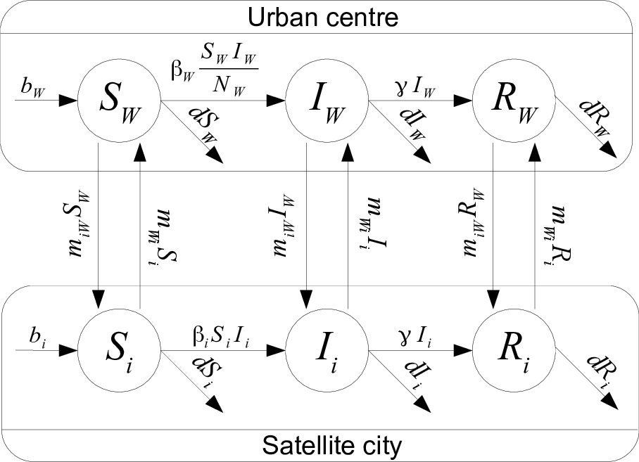
An urban centre and satellite cities
Context of the study
Winnipeg as urban centre and 3 smaller satellite cities: Portage la Prairie, Selkirk and Steinbach
- population density low to very low outside of Winnipeg
- MB road network well studied by MB Infrastructure Traffic Engineering Branch

Known and estimated quantities
| City | Pop. (2014) | Pop. (now) | Dist. | Avg. trips/day |
|---|---|---|---|---|
| Winnipeg (W) | 663,617 | 749,607 | - | - |
| Portage la Prairie (1) | 12,996 | 13,270 | 88 | 4,115 |
| Selkirk (2) | 9,834 | 10,504 | 34 | 7,983 |
| Steinbach (3) | 13,524 | 17,806 | 66 | 7,505 |
Estimating movement rates
Assume $m_{yx}$ movement rate from city $x$ to city $y$. Ceteris paribus, $N_x’=-m_{yx}N_x$, so $N_x(t)=N_x(0)e^{-m_{yx}t}$. Therefore, after one day, $N_x(1)=N_x(0)e^{-m_{yx}}$, i.e., \(m_{yx}=-\ln\left(\frac{N_x(1)}{N_x(0)}\right)\) Now, $N_x(1)=N_x(0)-T_{yx}$, where $T_{yx}$ number of individuals going from $x$ to $y$ / day. So \(m_{yx}=-\ln\left(1-\frac{T_{yx}}{N_x(0)}\right)\) Computed for all pairs $(W,i)$ and $(i,W)$ of cities
Sensitivity of $\mathcal{R}_0$ to variations of $\mathcal{R}_0^x\in[0.5,3]$
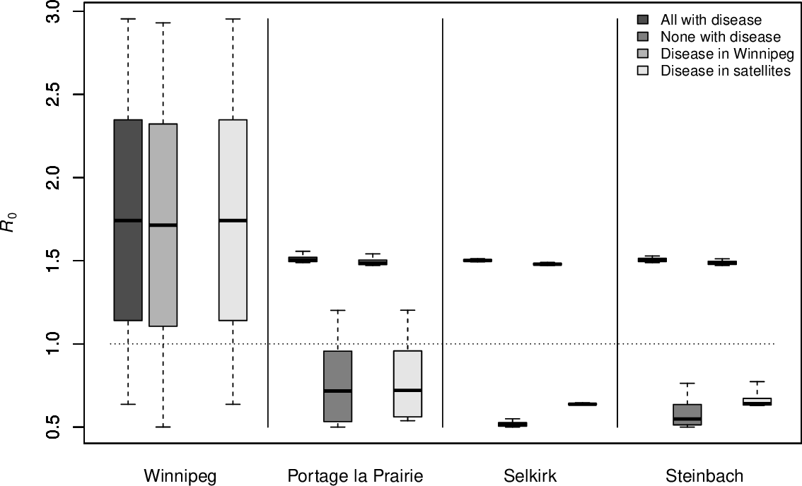 with disease: $\mathcal{R}_0^x=1.5$; without disease: $\mathcal{R}_0^x=0.5$. Each box and corresponding whiskers are 10,000 simulations
Lower connectivity can drive $\mathcal{R}_0$
PLP and Steinbach have comparable populations but with parameters used, only PLP can cause the general $\mathcal{R}_0$ to take values larger than 1 when $\mathcal{R}_0^W<1$
This is due to the movement rate: if $\mathcal{M}=0$, then \(\mathcal{R}_0=\max\{\mathcal{R}_0^W,\mathcal{R}_0^1,\mathcal{R}_0^2,\mathcal{R}_0^3\},\) since $FV^{-1}$ is then block diagonal
Movement rates to and from PLP are lower $\rightarrow$ situation closer to uncoupled case and $\mathcal{R}_0^1$ has more impact on the general $\mathcal{R}_0$
$\mathcal{R}_0$ does not tell the whole story!
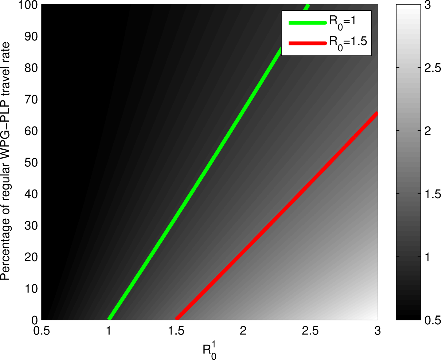
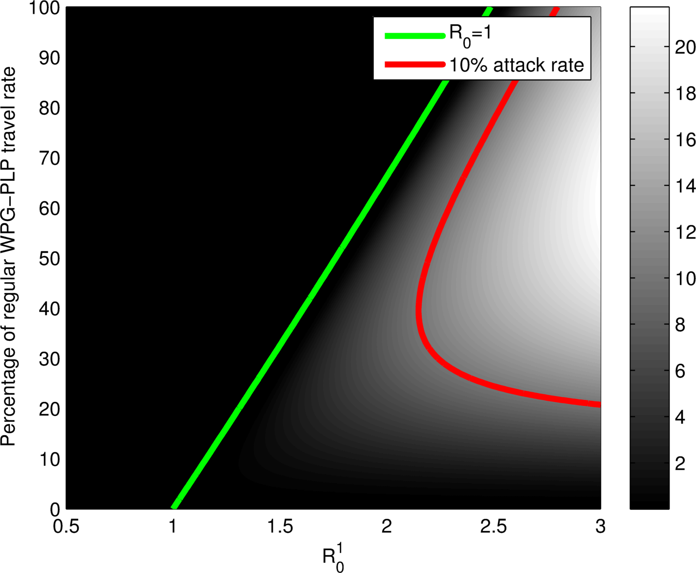 Plots as functions of $\mathcal{R}_0^1$ in PLP and the reduction of movement between Winnipeg and PLP. Left: general $\mathcal{R}_0$. Right: Attack rate in Winnipeg
Problems specific to metapopulations
Inherited dynamical properties (a.k.a. I am lazy)
Given \(\begin{align} s_{kp}' &= f_{kp}(S_p,I_p) \tag{9a} \label{sys:generic_intra_ds} \\ i_{\ell p}' &= g_{\ell p}(S_p,I_p) \tag{9b} \label{sys:generic_intra_di} \end{align}\) with known properties, what is known of \(\begin{align} s_{kp}' &= f_{kp}(S_p,I_p)+\textstyle{\sum_{q\in\mathcal{P}}} m_{kpq}s_{kq} \tag{10a} \label{sys:generic_inter_ds} \\ i_{\ell p}' &= g_{\ell p}(S_p,I_p)+\textstyle{\sum_{q\in\mathcal{P}}} m_{\ell pq}i_{\ell q} \tag{10b} \label{sys:generic_inter_di} \end{align}\)
- Existence and uniqueness $\checkmark$
- Invariance of $\mathbb{R}_+^\bullet$ under the flow $\checkmark$
- Boundedness $\checkmark$
- Location of individual $\mathcal{R}_{0i}$ and general $\mathcal{R}_0$?
- GAS?
An inheritance problem - Backward bifurcations
- Suppose a model that, isolated in a single patch, undergoes so-called backward bifurcations
- This means the model admits subthreshold endemic equilibria
- What happens when you couple many such consistuting units?
YES, coupling together backward bifurcating units can lead to a system-level backward bifurcation
JA, Ducrot & Zongo. A metapopulation model for malaria with transmission-blocking partial immunity in hosts. Journal of Mathematical Biology 64(3):423-448 (2012)
Metapopulation-induced behaviours ?
“Converse” problem to inheritance problem. Given \(\begin{align} s_{kp}' &= f_{kp}(S_p,I_p) \tag{9a} \\ i_{\ell p}' &= g_{\ell p}(S_p,I_p) \tag{9b} \end{align}\) with known properties, does \(\begin{align} s_{kp}' &= f_{kp}(S_p,I_p)+\textstyle{\sum_{q\in\mathcal{P}}} m_{kpq}s_{kq} \tag{10a} \\ i_{\ell p}' &= g_{\ell p}(S_p,I_p)+\textstyle{\sum_{q\in\mathcal{P}}} m_{\ell pq}i_{\ell q} \tag{10b} \end{align}\) exhibit some behaviours not observed in the uncoupled system?
E.g.: units have ${\mathcal{R}_0<1\implies$ DFE GAS, $\mathcal{R}_0>1\implies$ 1 GAS EEP$}$ behaviour, metapopulation has periodic solutions
Mixed equilibria
Can there be situations where some patches are at the DFE and others at an EEP?
This is the problem of mixed equilibria
This is a metapopulation-specific problem, not one of inheritance of dynamical properties!
Types of equilibria
Mixed equilibria
E.g., \(((S_1,I_1,R_1),(S_2,I_2,R_2))=((+,0,0),(+,+,+))\) is mixed, so is \(((S_1,I_1,R_1),(S_2,I_2,R_2))=((+,0,0),(+,0,+))\)
Note that MSAC $\implies$ $\mathcal{A}^c=\mathcal{A}$ and $\mathcal{D}^c=\mathcal{D}$ for all $c\in\mathcal{C}$
Interesting (IMHO) problems
More is needed on inheritance problem, in particular GAS part (Li, Shuai, Kamgang, Sallet, and older stuff: Michel & Miller, Šiljak)
Incorporate travel time (delay) and events (infection, recovery, death ..) during travel
What is the minimum complexity of the movement functions $m$ below \(\begin{aligned} s_{kp}' &= f_{kp}(S_p,I_p)+\textstyle{\sum_{q\in\mathcal{P}}} m_{kpq}(S,I)s_{kq} \\ i_{\ell p}' &= g_{\ell p}(S_p,I_p)+\textstyle{\sum_{q\in\mathcal{P}}} m_{\ell pq}(S,I)i_{\ell q} \end{aligned}\) required to observe a metapopulation-induced behaviour?
Global stability considerations
$|\mathcal{P}|$-SLIRS model
\[\begin{align} S_{p}' &=\mathcal{B}_p\left(N_p\right)+\nu_pR_p-\Phi_p-d_pS_p +\textstyle{\sum_{q\in\mathcal{P}}} m_{Spq}S_{q} \tag{2a} \\ L_{p}' &=\Phi_p-\left( \varepsilon_{p}+d_{p}\right)L_{p} +\textstyle{\sum_{q\in\mathcal{P}}} m_{Lpq}L_{q} \tag{2b} \\ I_{p}' &=\varepsilon_pL_p-(\gamma_p+d_p)I_p +\textstyle{\sum_{q\in\mathcal{P}}} m_{Ipq}I_{q} \tag{2c} \\ R_{p}' &=\gamma _{p}I_{p}-\left(\nu_{p}+d_{p}\right)R_{p} +\textstyle{\sum_{q\in\mathcal{P}}} m_{Rpq}R_{q} \tag{2d} \end{align}\] \[\Phi_p=\beta_p\frac{S_pI_p}{N_p} \tag{2e}\]The linear stability result for $\mathcal{R}_{0}<1$ can be strengthened to a global result
Proof
Since $S_{p}\leq N_{p},$ \(\Phi_p\leq\beta_p\frac{N_pI_p}{N_p}=\beta_p I_p\) and the equation for $\eqref{sys:pSLIRS_dL}$ gives the inequality \(\begin{equation} L_p' \leq \beta_pI_p-(\varepsilon_p+d_p)L_p+\sum_{q\in\mathcal{P}}m_{Lpq}L_{q} \label{eq:14} \end{equation}\) Define a linear system given by the equation above and $\eqref{sys:pSLIRS_dI}$ \(\begin{align*} L_p' &= \beta_pI_p-(\varepsilon_p+d_p)L_p+\sum_{q\in\mathcal{P}}m_{Lpq}L_q \\ I_p' &= \varepsilon_pL_p-(\gamma_p+d_p+\delta_p)I_p+\sum_{q\in\mathcal{P}}m_{Ipq}I_q \end{align*}\)
- This system linear has coefficient matrix $F-V$, and so (by some argument in the proof of local stability based on $\mathcal{R}0$) satisfies $\lim\limits{t\rightarrow \infty }L_{p}=0$ and $\lim\limits_{t\rightarrow \infty }I_{p}=0$ for $\mathcal{R}_{0}=\rho (FV^{-1})<1$
- Using a comparison theorem, it follows that these limits also hold for the nonlinear system in $\eqref{sys:pSLIRS_dL}$ and $\eqref{sys:pSLIRS_dI}$
- That $\lim\limits_{t\rightarrow \infty }R_{p}=0$ and $\lim\limits_{t\rightarrow \infty }S_{p}=N_{p}^\star$ follow from the equations for $\eqref{sys:pSLIRS_dS}$ and $\eqref{sys:pSLIRS_dR}$
Thus for $\mathcal{R}_{0}<1,$ the DFE is GAS and the disease dies out
$|\mathcal{S}|\;|\mathcal{P}|$-SLIRS (multiple species)
$\mathcal{S}$ a set of species \(\begin{align} S_{sp}' &= \mathcal{B}_{sp}(N_{sp})+\nu_{sp}R_{sp}-\Phi_{sp}-d_{sp}S_{sp} +\textstyle{\sum_{q\in\mathcal{P}}} m_{Sspq}S_{sq} \tag{3a} \\ L_{sp}' &= \Phi_{sp}-(\varepsilon_{sp}+d_{sp})L_{sp} +\textstyle{\sum_{q\in\mathcal{P}}}m_{Lspq}L_{sq} \tag{3b} \\ I_{sp}' &= \varepsilon_{sp}L_{sp}-(\gamma_{sp}+d_{sp})I_{sp} +\textstyle{\sum_{q\in\mathcal{P}}} m_{Ispq}I_{sq} \tag{3c} \\ R_{sp} &= \gamma _{sp}I_{sp}-(\nu_{sp}+d_{sp})R_{sp} +\textstyle{\sum_{q\in\mathcal{P}}} m_{Rspq}R_{sq} \tag{3d} \end{align}\)
\[\Phi_{sp}=\sum_{k\in\mathcal{S}}\beta_{skp}\frac{S_{sp}I_{kp}}{N_p} \tag{3e}\](Movement equal for all states: $m_{Xspq}=m_{spq}$ for $X\in{S,L,I,R}$)
Proof of the result
To establish the global stability of the DFE, consider the nonautonomous system consisting of $\eqref{sys:spSLIRS_dL}$, $\eqref{sys:spSLIRS_dI}$ and $\eqref{sys:spSLIRS_dR}$, with $\eqref{sys:spSLIRS_dL}$ written in the form \(\begin{equation}\label{sys:nonauton_E}\tag{11} \begin{aligned} L_{sp}' &= \sum_{j\in\mathcal{S}} \beta_{sjp}(N_{sp}-L_{sp}-I_{sp}-R_{sp})\frac{I_{jp}}{N_{jp}} \\ &\qquad -(d_{sp}+\varepsilon_{sp})L_{sp}+\sum_{q\in\mathcal{P}} m_{spq}L_{sq} \end{aligned} \end{equation}\) in which $S_{sp}$ has been replaced by $N_{sp}-L_{sp}-I_{sp}-R_{sp}$, and $N_{sp}$ is a solution of the equation for the total population \(\begin{equation} N_{sp}'=\sum_{q\in\mathcal{P}}m_{spq}N_{sq} \end{equation}\)
To continue, we need this
Write the system $\eqref{sys:nonauton_E}$, $\eqref{sys:spSLIRS_dI}$ and $\eqref{sys:spSLIRS_dR}$ as \(\begin{equation}\label{sys:nonauton} x' = f(t,x) \end{equation}\) where $x$ is the $3|\mathcal{S}||\mathcal{P}|$ dimensional vector consisting of the $L_{sp}$, $I_{sp}$ and $R_{sp}$
The DFE of the original system corresponds to the equilibrium $x=0$ in the the nonautonomous system
System for $N’$ can be solved for $N_{sp}(t)$ independently of the epidemic variables, and result earlier implies that the time dependent functions $N_{sp}(t)\to N^\star_{sp}$ as $t\to\infty$
Substituting this large time limit value $N_{sp}^\star$ for $N_{sp}$ in the nonautonomous equation $\eqref{sys:nonauton_E}$ for $L’$ gives
\(\begin{equation}\label{sys:asympt_auton_E}\tag{12}
\begin{aligned}
L_{sp}' =& \sum_{j\in\mathcal{S}}
\beta_{sjp}(N_{sp}^\star-L_{sp}-I_{sp}-R_{sp})\frac{I_{jp}}{N_{jp}^\star} \\
&-(d_{sp}+\varepsilon_{sp})L_{sp}+\sum_{q\in\mathcal{P}} m_{spq}L_{sq}
\end{aligned}
\end{equation}\)
Therefore, the nonautonomous system is asymptotically autonomous, with limit equation
\(\begin{equation}\label{sys:asympt_auton}
x' = g(x)
\end{equation}\)
To show that 0 is a globally asymptotically stable equilibrium for the limit system, consider the linear system \(\begin{equation}\label{sys:linear}\tag{13} x'=\mathcal{L}x \end{equation}\) where $x$ is the $3|\mathcal{S}||\mathcal{P}|$ dimensional vector consisting of the $L_{sp}$, $I_{sp}$ and $R_{sp}$. In $\mathcal{L}$, we replace $S_{sp}/N_{jp}$ with $N^\star_{sp}/N^\star_{jp}$. Equations $\eqref{sys:spSLIRS_dI}$ and $\eqref{sys:spSLIRS_dR}$ are not affected by this transformation, whereas $\eqref{sys:spSLIRS_dL}$ takes the form \(\begin{equation}\label{sys:lin_E}\tag{14} L_{sp}' = \sum_{j\in\mathcal{S}} \beta_{sjp}\frac{N_{sp}^\star}{N_{jp}^\star}I_{jp} -(d_{sp}+\varepsilon_{sp})L_{sp}+\sum_{q\in\mathcal{P}} m_{spq}L_{sq} \end{equation}\) Comparing $\eqref{sys:asympt_auton_E}$ and $\eqref{sys:lin_E}$, we note that $g(x)\leq\mathcal{L}x$ for all $x \in \mathbb{R}_+^{3|\mathcal{S}||\mathcal{P}|}$
In system $\eqref{sys:linear}$, the equations for $L_{sp}$ and $I_{sp}$ do not involve $R_{sp}$. Let $\tilde x$ be the part of the vector $x$ corresponding to the variables $E_{sp}$ and $I_{sp}$, and $\tilde{\mathcal{L}}$ be the corresponding submatrix of $\mathcal{L}$.
The method of used to prove local stability can also be applied to study the stability of the $\tilde x=0$ equilibrium of the subsystem $\tilde x’=\tilde{\mathcal{L}}\tilde x$, with $\tilde{\mathcal{L}}=F-V$
Therefore, if $\mathcal{R}0<1$, then the equilibrium $\tilde x=0$ of the subsystem $\tilde x’=\tilde{\mathcal{L}}\tilde x$ is stable. When $\tilde x=0$, $\eqref{sys:spSLIRS_dR}$ takes the form \(R_s' = (\mathcal{M}_s-D_s)R_s\) with $R_s=(R{s1},\ldots,R_{s|\mathcal{P}|})^T$ and $D_s=\mathsf{diag}(d_{s1},\ldots,d_{s|\mathcal{P}|})$
We know that $(-\mathcal{M}_s)$ is a singular M-matrix. It follows that $-\mathcal{M}_s+D_s$ is a nonsingular M-matrix for each $D_s$
Thus the equilibrium $R_s=0$ of the linear system in $R_s$ is stable
As a consequence, the equilibrium $x=0$ of $\eqref{sys:linear}$ is stable when $\mathcal{R}_0<1$
Using a standard comparison theorem, it follows that 0 is a globally asymptotically stable equilibrium of the asymptotically autonomous system $\eqref{sys:nonauton_E}$, $\eqref{sys:spSLIRS_dI}$ and $\eqref{sys:spSLIRS_dR}$
For $\mathcal{R}_0<1$, the linear system $\eqref{sys:lin_E}$-$\eqref{sys:spSLIRS_dI}$ has a unique equilibrium (the DFE) since its coefficient matrix $F-V$ is nonsingular
The proof of global stability is completed using results on asymptotically autonomous equations
Epilogue / Postlude
In conclusion
-
Space is a fundamental component of the epidemic spread process and cannot be ignored, both in modelling and in public health decision making
-
One way to model space is to use metapopulation models
-
Metapopulation models are easy to analyse locally, give interesting problems at the global level
-
We will see in Practicum 02 that simulation (deterministic and stochastic) can be costly in RAM and cycles but is easy
-
Metapopulation models are not the only solution!