3MC Course on Epidemiological Modelling
Course material (slides and code).
View the Project on GitHub julien-arino/3MC-course-epidemiological-modelling
Stochastic epidemic models
6 April 2022
Department of Mathematics & Data Science Nexus University of Manitoba*
Canadian Centre for Disease Modelling Canadian COVID-19 Mathematical Modelling Task Force NSERC-PHAC EID Modelling Consortium (CANMOD, MfPH, OMNI/RÉUNIS)
Outline
- Why stochasticity matters
- Discrete time Markov chains
- Continuous time Markov chains
Remarks / Resources
This is a user-oriented course: I barely, if at all, touch on the algorithms; instead, I focus on how to use them
Code is available in this Github repo in the CODE directory
Some of the slides are inspired from slides given to me by Linda Allen (Texas Tech). I recommend books and articles by Linda for more detail
- An Introduction to Stochastic Processes with Applications to Biology
- A primer on stochastic epidemic models: Formulation, numerical simulation, and analysis
Why stochasticity matters
Running example - SIS model without demography
Constant total population $P^\star$

Basic reproduction number: \(\mathcal{R}_0 = \dfrac{\beta}{\gamma}P^\star\)
In the deterministic world, $\mathcal{R}_0$ rules the world
- If $\mathcal{R}_0=\beta P^\star/\gamma<1$, the disease dies out (disease-free equilibrium)
- If $\mathcal{R}_0>1$, it becomes established at an endemic equilibrium $I^\star=P^\star-\gamma/\beta=(1-1/\mathcal{R}_0)P^\star$
Next slides: $P^\star = 100$K, $\gamma=1/5$, $\mathcal{R}_0={0.8,1.5,2.5}$ (and $\beta=\gamma \mathcal{R}_0/P^\star$)
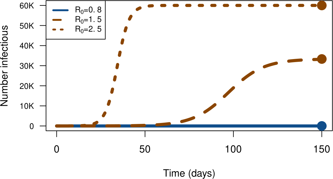
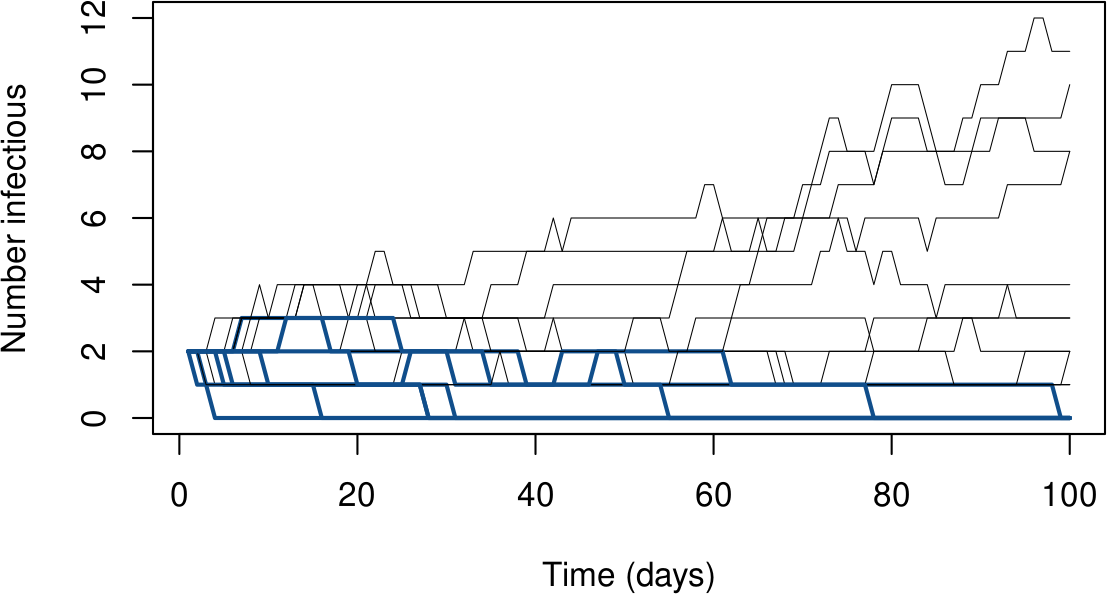
In stochastic world, make that ‘’$\mathcal{R}_0$ rules-ish’’ ($\mathcal{R}_0=1.5$)
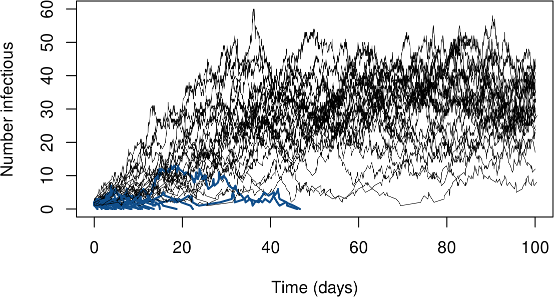
When $I_0=2$, extinctions happen quite frequently
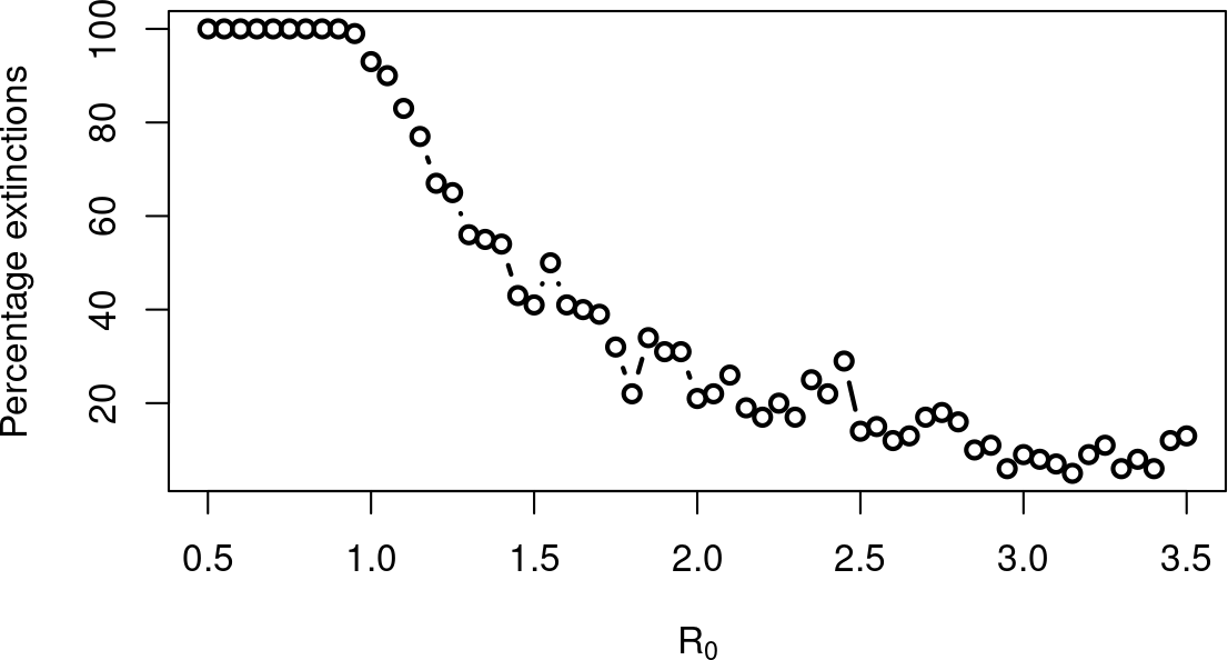
Types of stochastic systems discussed today
- Discrete-time Markov chains (DTMC)
- Continuous-time Markov chains (CTMC)
But there are many others. Of note:
- Branching processes (BP)
- Stochastic differential equations (SDE)
Discrete time Markov chains
Discrete-time Markov chains
$p(t)=(p_1(t),\ldots,p_n(t))^T$: probability vector, with $p_i(t)$ describing the probability that at time $t$, the system is in state $S_i$, $i=1,\ldots,n$
$\sum_i p_i(t)=1$ for al# l $t$, of course
State evolution governed by \(p(t+\Delta t) = A(\Delta t)p(t)\) where $A(\Delta t)$ is a stochastic matrix (row sums all equal 1), the transition matrix, with entry $a_{ij}=\mathbb{P}(X_{t+\Delta t}=s_i|X_t=s_j)$, where $X_1,\ldots$ sequence of random variables describing the state
If $A(\Delta t)=A$ constant, homogeneous DTMC
Time often ‘‘recast’’ so that $\Delta t=1$
Important remark
The DTMC world lives at the interface between probabilists, who like to think of $p(t)$ as a row vector, $A(\Delta t)$ as a column-stochastic matrix and thus write \(p(t+\Delta t) = p(t)A(\Delta t)\) and linear algebraists, who prefer column vectors and row-stochastic matrices, \(p(t+\Delta t) = A(\Delta t)p(t)\)
So check the direction to understand whether you are using $A$ or $A^T$
Advantages of DTMC
As a teacher of modelling: base theory of DTMC uses a lot of linear algebra and graph theory; usually really appreciated by students
Regular DTMC (with primitive transition matrices) allow to consider equilibrium distribution of probability
Absorbing DTMC (with reducible transition matrices) allow the consideration of time to absorption, mean first passage time, etc.
See for instance book of Kemeny and Snell
DTMC for example SIS system
Since $S=P^\star-I$, consider only the infected. To simulate as DTMC, consider a random walk on $I$ ($\simeq$ Gambler’s ruin problem)
Denote $\lambda_I = \beta (P^\star-I)I\Delta t$, $\mu_I = \gamma I\Delta t$ and $\sigma_I=1-(\lambda_I+\mu_I)\Delta t$

Transition matrix
\[A = \begin{pmatrix} 1 & 0 \\ \mu_1 & \sigma_1 & \lambda_1 & 0 \\ 0 & \mu_2 & \sigma_2 & \lambda_2 & 0 \\ \\ & & & & & \ddots \\ \\ & & & & & & 0 & \mu_{P^\star-1} & \mu_{P^\star-1} & \lambda_{P^\star-1} & 0 \\ &&&&&&&& 0 & \mu_{P^\star} & \sigma_{P^\star} \end{pmatrix}\]# Make the transition matrix
T = mat.or.vec(nr = (Pop+1), nc = (Pop+1))
for (row in 2:Pop) {
I = row-1
mv_right = gamma*I*Delta_t # Recoveries
mv_left = beta*I*(Pop-I)*Delta_t # Infections
T[row,(row-1)] = mv_right
T[row,(row+1)] = mv_left
}
# Last row only has move left
T[(Pop+1),Pop] = gamma*(Pop)*Delta_t
# Check that we don't have too large values
if (max(rowSums(T))>1) {
T = T/max(rowSums(T))
}
diag(T) = 1-rowSums(T)
Simulating a DTMC
library(DTMCPack)
sol = MultDTMC(nchains = 20, tmat = T, io = IC, n = t_f)
gives 20 realisations of a DTMC with transition matrix T, initial conditions IC (a vector of initial probabilities of being in the different $I$ states) and final time t_f
See code on Github
Going a bit further
DTMCPack is great for obtaining realisations of a DTMC, but to study it in more detail, markovchain is much more comprehensive
library(markovchain)
mcSIS <- new("markovchain",
             states = sprintf("I_%d", 0:Pop),
             transitionMatrix = T,
             name = "SIS")
Note that interestingly, markovchain overrides the weird default “* is Hadamard, %*% is usual” R matrix product rule, so mcSIS*mcSIS does $TT$, not $T\circ T$
> summary(mcSIS)
SIS  Markov chain that is composed by:
Closed classes:
I_0
Recurrent classes:
{I_0}
Transient classes:
{I_1,I_2,I_3,I_4,I_5,I_6,I_7,I_8,I_9,I_10,I_11,I_12,I_13,I_14,I_15,
I_16,I_17,I_18,I_19,I_20,I_21,I_22,I_23,I_24,I_25,I_26,I_27,I_28,
I_29,I_30,I_31,I_32,I_33,I_34,I_35,I_36,I_37,I_38,I_39,I_40,I_41,
I_42,I_43,I_44,I_45,I_46,I_47,I_48,I_49,I_50,I_51,I_52,I_53,I_54,
I_55,I_56,I_57,I_58,I_59,I_60,I_61,I_62,I_63,I_64,I_65,I_66,I_67,
I_68,I_69,I_70,I_71,I_72,I_73,I_74,I_75,I_76,I_77,I_78,I_79,I_80,
I_81,I_82,I_83,I_84,I_85,I_86,I_87,I_88,I_89,I_90,I_91,I_92,I_93,
I_94,I_95,I_96,I_97,I_98,I_99,I_100}
The Markov chain is not irreducible
The absorbing states are: I_0
| Function | Role |
|---|---|
absorbingStates |
absorbing states of the transition matrix, if any |
steadyStates |
the vector(s) of steady state(s) in matrix form |
meanFirstPassageTime |
matrix or vector of mean first passage times |
meanRecurrenceTime |
vector of mean number of steps to return to each recurrent state |
hittingProbabilities |
matrix of hitting probabilities for a Markov chain |
meanAbsorptionTime |
expected number of steps for a transient state to be absorbed by any recurrent class |
absorptionProbabilities |
$\mathbb{P}$ transient states being absorbed by each recurrent state |
canonicForm |
canonic form of transition matrix |
period |
the period of an irreducible DTMC |
summary |
DTMC summary |
</span>
Continuous time Markov chains
Continuous-time Markov chains
CTMC similar to DTMC except in way they handle time between events (transitions)
DTMC: transitions occur each $\Delta t$
CTMC: $\Delta t\to 0$ and transition times follow an exponential distribution parametrised by the state of the system
CTMC are roughly equivalent to ODE
ODE to CTMC : focus on different components
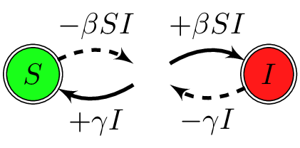
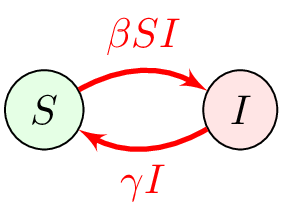
| Weight | Transition | Effect |
|---|---|---|
| $\beta SI$ | $S\to S-1$, $I\to I+1$ | new infection of a susceptible |
| $\gamma I$ | $S\to S+1$, $I\to I-1$ | recovery of an infectious |
Will use $S=N^*-I$ and omit $S$ dynamics
Gillespie’s algorithm (SIS model with only I eq.)
set $t\leftarrow t_0$ and $I(t)\leftarrow I(t_0)$ while {$t\leq t_f$}
- $\xi_t\leftarrow \beta (P^\star-i)i+\gamma i$
- Draw $\tau_t$ from $T\thicksim \mathcal{E}(\xi_t)$
- $v\leftarrow\left[\beta (P^\star-i)i,\xi_t\right]/\xi_t$
- Draw $\zeta_t$ from $\mathcal{U}([0,1])$
- Find $pos$ such that $v_{pos-1}\leq\zeta_t\leq v_{pos}$
- switch {$pos$}
- 1: New infection, $I(t+\tau_t)=I(t)+1$
- 2: End of infectious period, $I(t+\tau_t)=I(t)-1$
- $t\leftarrow t+\tau_t$
You can also use a package
- You can implement Gillespie’s algorithm yourself, it is a good exercise..
- But in R there also exists a few packages allowing you to do that easily
- They have the advantage of implementing tau-leaping (more on this later)
Simulating a CTMC
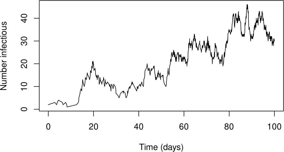
library(GillespieSSA2)
IC <- c(S = (Pop-I_0), I = I_0)
params <- c(gamma = gamma, beta = beta)
reactions <- list(
  reaction("beta*S*I", c(S=-1,I=+1), "new_infection"),
  reaction("gamma*I", c(S=+1,I=-1), "recovery")
)
set.seed(NULL)
sol <- ssa(
    initial_state = IC,
    reactions = reactions,
    params = params,
    method = ssa_exact(),
    final_time = t_f,
)
plot(sol$time, sol$state[,"I"], type = "l",
     xlab = "Time (days)", ylab = "Number infectious")
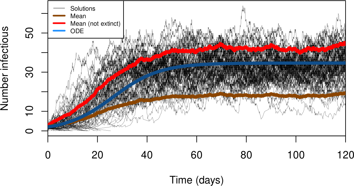
Sometimes in a CTMC things go bad
- Recall that the inter-event time is exponentially distributed
- Critical step of the Gillespie algorithm:
- $\xi_t\leftarrow$ weight of all possible events (propensity)
- Draw $\tau_t$ from $T\thicksim \mathcal{E}(\xi_t)$
- So the inter-event time $\tau_t\to 0$ if $\xi_t$ becomes very large for some $t$
- This can cause the simulation to grind to a halt
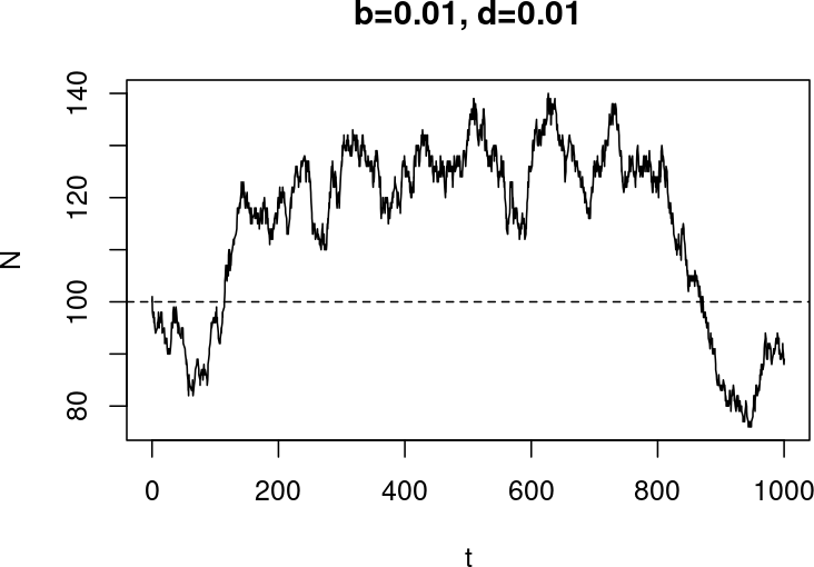
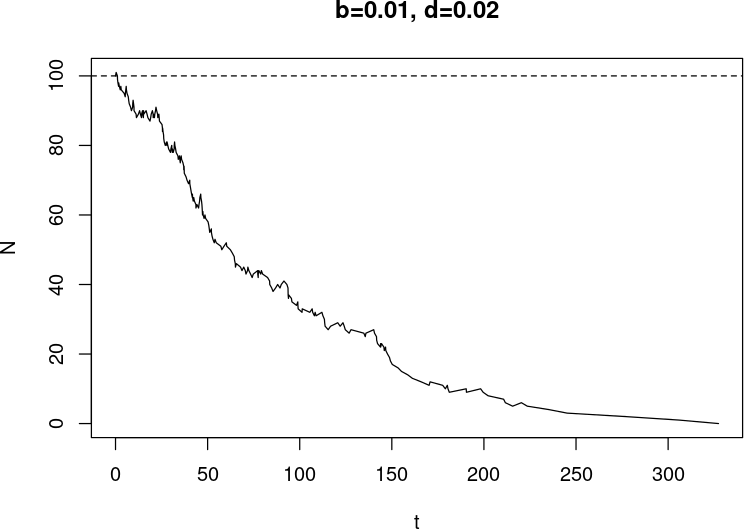
Example: a birth and death process
- Individuals born at per capita rate $b$
- Individuals die at per capita rate $d$
- Let’s implement this using classic Gillespie
Gillespie’s algorithm (birth-death model)
set $t\leftarrow t_0$ and $N(t)\leftarrow N(t_0)$ while {$t\leq t_f$}
- $\xi_t\leftarrow (b+d)N(t)$
- Draw $\tau_t$ from $T\thicksim \mathcal{E}(\xi_t)$
- $v\leftarrow\left[bN(t),\xi_t\right]/\xi_t$
- Draw $\zeta_t$ from $\mathcal{U}([0,1])$
- Find $pos$ such that $v_{pos-1}\leq\zeta_t\leq v_{pos}$
- switch {$pos$}
- 1: Birth, $N(t+\tau_t)=N(t)+1$
- 2: Death, $N(t+\tau_t)=N(t)-1$
- $t\leftarrow t+\tau_t$
b = 0.01   # Birth rate
d = 0.01   # Death rate
t_0 = 0    # Initial time
N_0 = 100  # Initial population

# Vectors to store time and state. Initialise with initial condition.
t = t_0
N = N_0

t_f = 1000  # Final time

# We'll track the current time and state (could also just check last entry in t
# and N, but will take more operations)
t_curr = t_0
N_curr = N_0
while (t_curr<=t_f) {
  xi_t = (b+d)*N_curr
  # The exponential number generator does not like a rate of 0 (when the
  # population crashes), so we check if we need to quit
  if (N_curr == 0) {
    break
  }
  tau_t = rexp(1, rate = xi_t)
  t_curr = t_curr+tau_t
  v = c(b*N_curr, xi_t)/xi_t
  zeta_t = runif(n = 1)
  pos = findInterval(zeta_t, v)+1
  switch(pos,
         {
           # Birth
           N_curr = N_curr+1
         },
         {
           # Death
           N_curr = N_curr-1
         })
  N = c(N, N_curr)
  t = c(t, t_curr)
}
Drawing at random from an exponential distribution
If you do not have an exponential distribution random number generator.. We want $\tau_t$ from $T\thicksim\mathcal{E}(\xi_t)$, i.e., $T$ has probability density function \(f(x,\xi_t)= \xi_te^{-\xi_t x}\mathbf{1}_{x\geq 0}\) Use cumulative distribution function $F(x,\xi_t)=\int_{-\infty}^x f(s,\xi_t)\,ds$ \(F(x,\xi_t)= (1-e^{-\xi_t x})\mathbf{1}_{x\geq 0}\) which has values in $[0,1]$. So draw $\zeta$ from $\mathcal{U}([0,1])$ and solve $F(x,\xi_t)=\zeta$ for $x$ \(\begin{align*} F(x,\xi_t)=\zeta & \Leftrightarrow 1-e^{-\xi_tx}=\zeta \\ &\Leftrightarrow e^{-\xi_tx} = 1-\zeta \\ &\Leftrightarrow \xi_tx = -\ln(1-\zeta) \\ &\Leftrightarrow \boxed{x = \frac{-\ln(1-\zeta)}{\xi_t}} \end{align*}\)
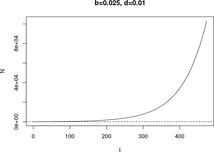
Last one did not go well
- Wanted 1000 time units (days?)
- Interrupted around 500 ($t=473.4544$) because I lost patience
- (Slide before: the sim stopped because the population went extinct, I did not stop it!)
- At stop time
-
$ N = 241,198$ (and $ t $ as well, of course!) - time was moving slowly
> tail(diff(t))
[1] 1.357242e-04 1.291839e-04 5.926044e-05 7.344020e-05 1.401148e-04 4.423529e-04
-

Tau-leaping to the rescue!
- Will not go into details
- Approximation method (compared to classic Gillespie, which is exact)
- Roughly: consider “groups” of events instead of individual events
- Good news:
GillespieSSA2(which we saw earlier) andadaptivetau