R for modellers - Vignette 08

Acquiring data

Julien Arino

Department of Mathematics

University of Manitoba*

* The University of Manitoba campuses are located on original lands of Anishinaabeg, Cree, Oji-Cree, Dakota and Dene peoples, and on the homeland of the Métis Nation.

Outline

• Be “data aware”
• Data is everywhere
• Data gathering methods
• Example - Dutch Elm Disease
• Example: population of South Africa

Be “data aware”

Be data aware

• Using R (or Python), it is really easy to grab data from the web, e.g., from Open Data sources
• More and more locations have an open data policy
• As a modeller, you do not need to have data everywhere, but you should be aware of the context
• If you want your work to be useful, for instance in public health, you cannot be completely disconnected from reality

Data is everywhere

Closed data

• Often generated by companies, governments or research labs
• When available, come with multiple restrictions

Open data

• Often generated by the same entities but “liberated” after a certain period
• More and more frequent with governments/public entities
• Wide variety of licenses, so beware
• Wide variety of qualities, so beware

Open Data initiatives

Recent movement (5-10 years): governments (local or higher) create portals where data are centralised and published

• Winnipeg
• Alberta
• Canada
• Europe
• UN
• World Bank
• WHO

Data gathering methods

• Example: population of South Africa
• Example - Dutch Elm Disease
• Data wrangling

• JA. Mathematical epidemiology in a data-rich world. Infectious Disease Modelling 5:161-188 (2020)
• See also GitHub repo for that paper

Data gathering methods

• By hand
• Using programs such as Engauge Digitizer or g3data
• Using natural language processing and other web scraping methods
• Using APIs
• Using R or Python packages (to interface with APIs)

Example - Dutch Elm Disease

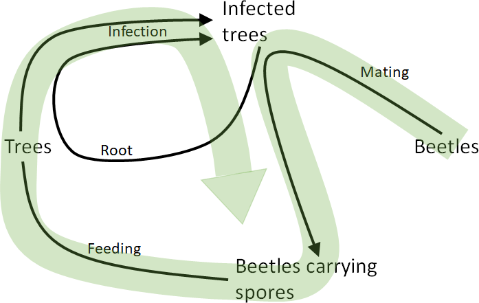
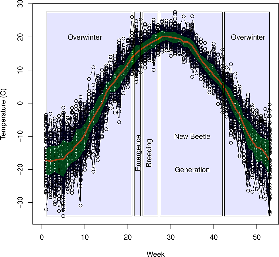
Dutch Elm Disease

• Fungal disease that affects Elms
• Caused by the fungus Ophiostoma ulmi
• Transmitted by the Elm bark beetle (Scolytus scolytus)
• Has decimated North American urban elm forests

bg contain

bg contain

bg contain

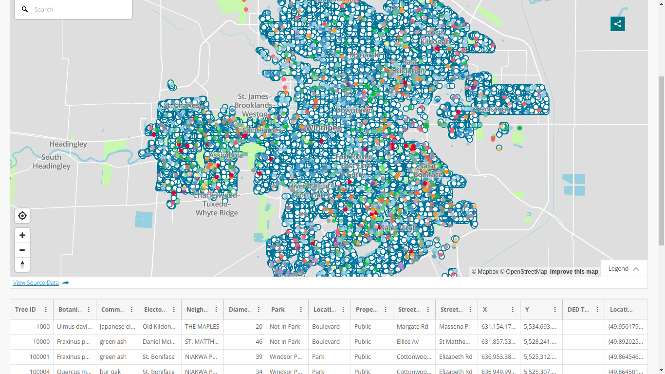
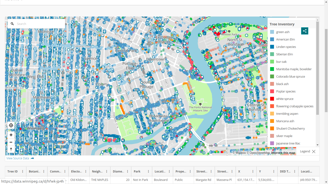
Getting the tree data

allTrees = read.csv("https://data.winnipeg.ca/api/views/hfwk-jp4h/ro

After this,

dim(allTrees)
## [1] 300846
15

Let us clean things a little

elms_idx = grep("American Elm", allTrees$Common.Name, ignore.case = TRUE)
elms = allTrees[elms_idx, ]

We are left with 54,036 American elms

bg contain

bg contain

Computation of root systems interactions

(Needs a relatively large machine here - about 50GB RAM)

• If roots of an infected tree touch roots of a susceptible tree, fungus is transmitted
• Spread of a tree’s root system depends on its height (we have diametre at breast height, DBH, for all trees)
• The way roadways are built, there cannot be contacts between root systems of trees on opposite sides of a street

Distances between all trees

elms_xy = cbind(elms$X, elms$Y)
D = dist(elms_xy)
idx_D = which(D<50)

indices_LT is a large \(N(N-1)/2\times 2\) matrix with indices (orig,dest) of trees in the pairs of elms, so indices_LT[idx_D] are the pairs under consideration

Keep a little more..

indices_LT_kept = as.data.frame(cbind(indices_LT[idx_D,],
                                D[idx_D]))
colnames(indices_LT_kept) = c("i","j","dist")

Create line segments between all pairs of trees

tree_locs_orig = cbind(elms_latlon$lon[indices_LT_kept$i],
                       elms_latlon$lat[indices_LT_kept$i])
tree_locs_dest = cbind(elms_latlon$lon[indices_LT_kept$j],
                       elms_latlon$lat[indices_LT_kept$j])
tree_pairs = do.call(
  sf::st_sfc,
  lapply(
    1:nrow(tree_locs_orig),
    function(i){
      sf::st_linestring(
        matrix(
          c(tree_locs_orig[i,],
            tree_locs_dest[i,]), 
          ncol=2,
          byrow=TRUE)
      )
    }
  )
)

A bit of mapping

library(tidyverse)
# Get bounding polygon for Winnipeg
bb_poly = osmdata::getbb(place_name = "winnipeg", 
                         format_out = "polygon")
# Get roads
roads <- osmdata::opq(bbox = bb_poly) %>%
  osmdata::add_osm_feature(key = 'highway', 
                           value = 'residential') %>%
  osmdata::osmdata_sf () %>%
  osmdata::trim_osmdata (bb_poly)
# Get rivers
rivers <- osmdata::opq(bbox = bb_poly) %>%
  osmdata::add_osm_feature(key = 'waterway', 
                           value = "river") %>%
  osmdata::osmdata_sf () %>%
  osmdata::trim_osmdata (bb_poly)

And we finish easily

• We have the pairs of trees potentially in contact with each other
• We have the roads and rivers of the city, which is a collection of line segments
• If there is an intersection between a tree pair and a road/river, then we can forget this tree pair as their root systems cannot come into contact

st_crs(tree_pairs) = sf::st_crs(roads$osm_lines$geometry)
iroads = sf::st_intersects(x = roads$osm_lines$geometry,
                           y = tree_pairs)
irivers = sf::st_intersects(x = rivers$osm_lines$geometry,
                            y = tree_pairs)

tree_pairs_roads_intersect = c()
for (i in 1:length(iroads)) {
  if (length(iroads[[i]])>0) {
    tree_pairs_roads_intersect = c(tree_pairs_roads_intersect,
                                   iroads[[i]])
  }
}
tree_pairs_roads_intersect = sort(tree_pairs_roads_intersect)
to_keep = 1:dim(tree_locs_orig)[1]
to_keep = setdiff(to_keep,tree_pairs_roads_intersect)

bg contain

Example: population of South Africa

library(wbstats)
pop_data_CTRY <- wb_data(country = "ZAF", indicator = "SP.POP.TOTL",
                         mrv = 100, return_wide = FALSE)
y_range = range(pop_data_CTRY$value)
y_axis <- make_y_axis(y_range)
png(file = "pop_ZAF.png", 
    width = 800, height = 400)
plot(pop_data_CTRY$date, pop_data_CTRY$value * y_axis$factor,
     xlab = "Year", ylab = "Population", type = "b", lwd = 2,
     yaxt = "n")
axis(2, at = y_axis$ticks, labels = y_axis$labels, las = 1)
dev.off()
crop_figure("pop_ZAF.png")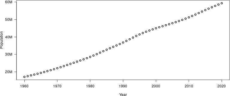

bg contain