R for modellers - Vignette 10

Solving ODE in R

Julien Arino

Department of Mathematics

University of Manitoba*

* The University of Manitoba campuses are located on original lands of Anishinaabeg, Cree, Oji-Cree, Dakota and Dene peoples, and on the homeland of the Métis Nation.

The deSolve library

As already pointed out, deSolve:

The functions provide an interface to the FORTRAN functions ‘lsoda’, ‘lsodar’, ‘lsode’, ‘lsodes’ of the ‘ODEPACK’ collection, to the FORTRAN functions ‘dvode’, ‘zvode’ and ‘daspk’ and a C-implementation of solvers of the ‘Runge-Kutta’ family with fixed or variable time steps

You are benefiting from years and years of experience: ODEPACK is a set of Fortran (77!) solvers developed at Lawrence Livermore National Laboratory (LLNL) starting in the late 70s

Other good solvers written in C are also included

Refer to the package help for details

Using deSolve for simple ODEs

As with most numerical solvers, you need to write a function returning the value of the right hand side of your equation (the vector field) at a given point in phase space, then call this function from the solver

First, we load the library

library(deSolve)

The required ingredients

A function describing the right hand side of the differential equation
Initial conditions
Times at which to return the value of the solution
(Optional) Parameters

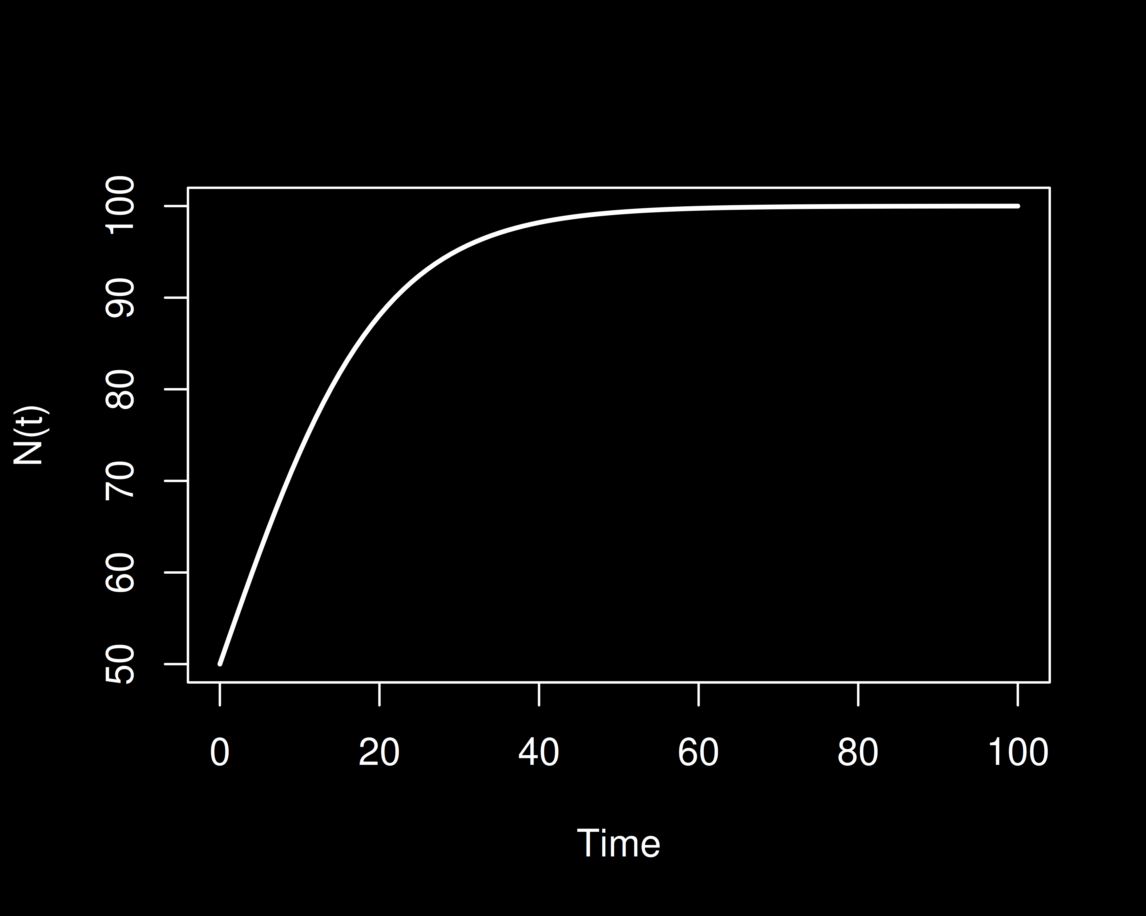
Example - the logistic ODE

The logistic ODE

\[ \frac{d}{dt}N(t)= rN(t)\left(1-\frac{N(t)}{K}\right) \] or, omitting time dependence \[ N' = rN\left(1-\frac NK\right) \]

$r$ growth rate
$K$ carrying capacity
$N(0)\geq 0$ initial condition

IC / times / parameters

IC = c(N = 50)
times = seq(0, 100, 1)
params = list(r = 0.1, K = 100)

IC is a named vector
times is a vector of times at which the solution is returned (not necessarily where it is computed, can be different from this)
params is a list

The right hand side function (v1)

rhs_logistic_v1 <- function(t, x, p) {
  dN <- p$r * x[1] *(1-x[1]/p$K)
  return(list(dN))
}

The right hand side function (v2)

rhs_logistic_v2 <- function(t, x, p) {
  with(as.list(x), {
    dN <- p$r * N *(1-N/p$K)
    return(list(dN))
  })
}

The right hand side function (v3)

rhs_logistic_v3 <- function(t, x, p) {
  with(as.list(c(x, p)), {
    dN <- r * N *(1-N/K)
    return(list(dN))
  })
}

In this case, beware of not having a variable and a parameter with the same name..

Just to clarify:

as.list(c(IC, params))

$N
[1] 50

$r
[1] 0.1

$K
[1] 100

and using with(as.list(c())) makes these values available to the function with just the names (hence we do not need p$r, for instance)

Finally, call the solver

sol_v1 <- ode(IC, times, rhs_logistic_v1, params)
sol_v2 <- ode(IC, times, rhs_logistic_v2, params)
sol_v3 <- ode(IC, times, rhs_logistic_v3, params)

Just to make sure results are the same

any(sol_v1 != sol_v2)

[1] FALSE

any(sol_v1 != sol_v3)

[1] FALSE

any(sol_v2 != sol_v3)

[1] FALSE

What a solution looks like

head(sol_v1, n = 8)

     time        N
[1,]    0 50.00000
[2,]    1 52.49788
[3,]    2 54.98347
[4,]    3 57.44433
[5,]    4 59.86886
[6,]    5 62.24604
[7,]    6 64.56573
[8,]    7 66.81887

Plot the result

plot(sol_v1[,"time"], sol_v1[,"N"],
     xlab = "Time", ylab = "N(t)",
     type = "l", lwd = 2)

Changing integration parameters

Default method: `lsoda`

lsoda switches automatically between stiff and nonstiff methods
You can also specify other methods: “lsode”, “lsodes”, “lsodar”, “vode”, “daspk”, “euler”, “rk4”, “ode23”, “ode45”, “radau”, “bdf”, “bdf_d”, “adams”, “impAdams” or “impAdams_d” ,“iteration” (the latter for discrete-time systems)

ode(y, times, func, parms, method = "ode45")

You can implement your own integration method