When working with students and postdocs, I often provide “skeletons”, i.e., canonical examples of code that illustrate something that I want them to do in another context. Example: running some code in parallel. Here, I will carry out a very simple and naive sensitivity analysis of the value of the basic reproduction number \(\mathcal{R}_0\) in the basic Kermack and McKendrick SIR model.

First, we need the function that we will evaluate for a given point in parameter space. Note that we pass parameters as a list rather than an ordered t-uple of parameters; this allows to not have to worry about the order in which parameters are presented.

R0 = function(p) {
  return(p$beta*p$S0/p$gamma)
}

The following function converts one or several parameter values given in the list by lapply or parLapply into a value of \(\mathcal{R}_0\). Note the little trick, which allows to set as many parameters as are provided in the element of the list received as argument.

one_run_R0 = function(p,param) {
  for (pp in names(p))
    param[[pp]] = p[[pp]]
  return(R0(param))
}

Set up parameters by default. If not changed by the function above, they take these values.

param = list()
param$beta = 1e-6
param$S0 = 10000
param$gamma = 1/4.5 # Average duration of infection

Set up the list of parameters that are going to vary. For illustration, we do 10,000 computations for varying values of \(\beta\), 10,000 for varying values of \(S_0\) and 10,000 simulations for varying values of both \(\beta\) and \(S_0\).

nb_sims = 10000 # nb of simulations of each type
param_vary = list()
for (i in 1:nb_sims) {
  param_vary[[i]] = list()
  param_vary[[i]]$beta = runif(1, min = 1e-9, max = 1e-4)
}
for (i in (nb_sims+1):(2*nb_sims)) {
  param_vary[[i]] = list()
  param_vary[[i]]$S0 = runif(1, min = 1000, max = 100000)
}
for (i in (2*nb_sims+1):(3*nb_sims)) {
  param_vary[[i]] = list()
  param_vary[[i]]$beta = runif(1, min = 1e-9, max = 1e-4)
  param_vary[[i]]$S0 = runif(1, min = 1000, max = 100000)
}

The code can be run in parallel or iteratively. Note one interesting quirk: the function argument to parLapply is called fun, while that to lapply is called FUN. You have to love R. One core is set aside to avoid rendering the computer completely unresponsive; on a cluster with head node, you would of course be able to devote all cores to computations. (But then again, on a cluster with head node, you might also be using a scheduler.)

RUN_PARALLEL = TRUE
if (RUN_PARALLEL) {
  # Detect number of cores, use all but 1
  no_cores <- parallel::detectCores() - 1
  # Initiate cluster
  tictoc::tic()
  cl <- parallel::makeCluster(no_cores)
  # Export needed variables
  parallel::clusterExport(cl,
                c("R0",
                  "one_run_R0",
                  "param"))
  # Run computation
  result = parallel::parLapply(cl = cl, X = param_vary,
                               fun =  function(x) one_run_R0(x,param))
  # Stop cluster
  parallel::stopCluster(cl)
  tictoc::toc()
} else {
  tictoc::tic()
  result = lapply(X = param_vary,
                  FUN = function(x) one_run_R0(x,param))
  tictoc::toc()
}

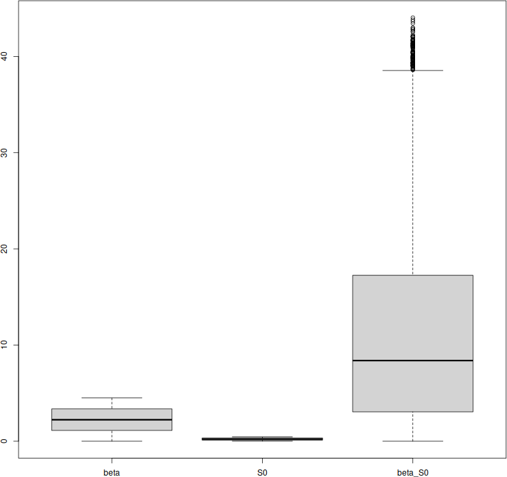
Last little piece: let us plot the range of values taken by \(\mathcal{R}_0\) when the various parameters are varied, to show sensitivity of \(\mathcal{R}_0\).

result = unlist(result)
result.df = data.frame(beta = result[1:nb_sims],
                       S0 = result[(nb_sims+1):(2*nb_sims)],
                       beta_S0 = result[(2*nb_sims+1):(3*nb_sims)])
boxplot(result.df)