Spatio-temporal spread of diseases
dynamics of metapopulation disease models
Diseases are mobile creatures
The earliest reference I know to the spatio-temporal spread of infectious diseases is in the History of the Peloponnesian War, by Thucydides (460-395 BC). In this passage (link), Thucydides describes the arrival into Athens of a “plague” circa 430 BC:
It first began, it is said, in the parts of Ethiopia above Egypt, and thence descended into Egypt and Libya and into most of the king’s country. Suddenly falling upon Athens, it first attacked the population in Piraeus,—which was the occasion of their saying that the Peloponnesians had poisoned the reservoirs, there being as yet no wells there—and afterwards appeared in the upper city, when the deaths became much more frequent.
The king referred to in the text is the Persian king Artaxerxes I; at the time, the Persian Empire (or Achaemenid Empire) covered an extensive region (map) and dominated most of the “known world”. While the epidemic was originally thought to be a plague, recent work has established that it probably was typhus. See this blog entry I wrote about Thucydides.
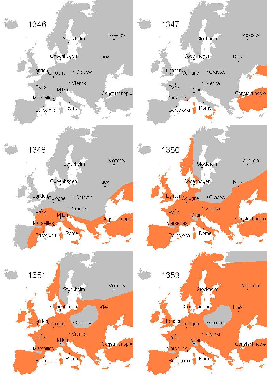
Skip forward more than 1500 years. In medieval and renaissance Europe, a succession of plagues caused extensive death, starting with the most devastating of all, the Black Death, which from 1346 to 1353 wiped out an estimated 30 to 60% of the population of Europe at the time. The spatio-temporal spread of the infection is clearly visible in this picture:

Plagues continued to hit western and central Europe until the mid-1750s, with the last major events the Great Plague of Marseille of 1720-1722, the Great Plague of 1738 in the Balkans and the Plague of Messina in 1743.
Evolution of spreading patterns for human diseases
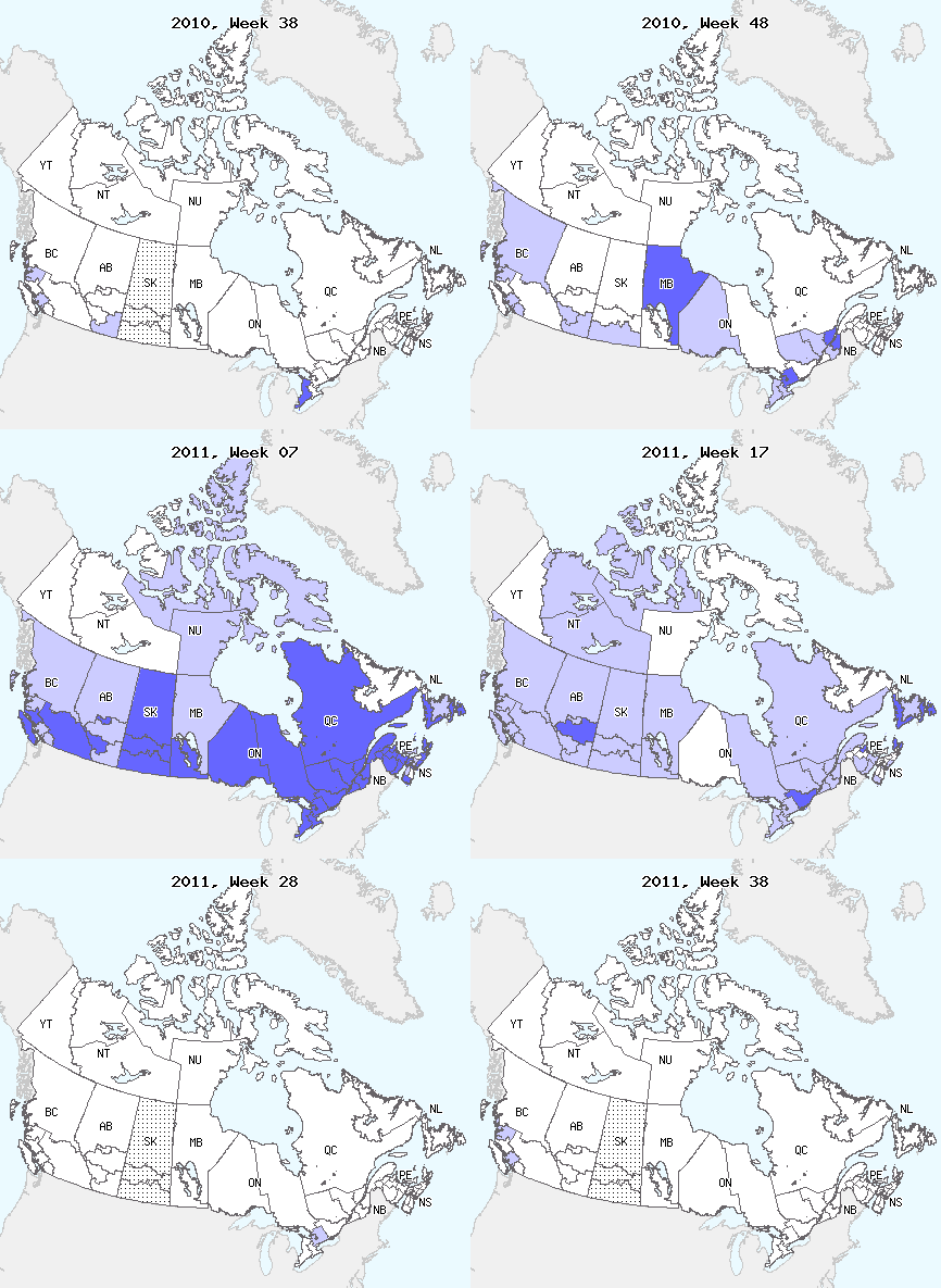
Compare the patterns of spread of infection for the Black Plague in Europe in the 1350s and Influenza in Canada in 2010-2011 in the figures below.


While the spatial spread of animal diseases still often follow the same type of pattern, disease for which the main carrier is human have evolved considerably since the plagues. While Black Death exhibited a travelling wavefront of infection, modern day Influenza seems to follow a mostly random pattern, with some degree of “nearest neighbour” propagation combined with more long range propagation (and establishment) events.
The main reason for this change of pattern is the fantastic evolution of transport since then. An example among many illustrates this evolution. In Histoire de la maison de Bourbon, published in 1786, Joseph-Louis Ripault Desormeaux explains that Jeanne d’Albret, mother of the future king Henri IV of France, had promised her father, Henri II of Navarre, that her son would be born in Pau, in the southwest of France. The trip, which took place in 1553, is described as follows.
Les deux époux séjournèrent quelques mois à la Flèche; là, dit-on, fut conçu Henri IV; ensuite ils se rendirent fur la frontière de Picardie, où ils restèrent jusqu’au mois de Décembre, que Jeanne d’Albret prit congé d’Antoine de Bourbon: elle étoit grosse alors de huit mois; elle traverfa toute la France, depuis Compiegne jusqu’aux monts Pyrénées, & arriva dans la Capitale du Béarn : son voyage n’avoit été que de dix-huit jours.
(The two spouses spent several months in la Flèche; there, it is said, is where Henri IV conceived; then they went to the border of Picardie, where they remained until December, that Jeanne d’Albret left Antoine de Bourbon: she was then eight months pregnant; she travelled through France, from Compiegne to the Pyrenees mountains, & arrived in the capital of Bearn: her trip had only lasted eighteen days.)
By comparison, it now takes 5 hours by high speed train (TGV) or 1 hour by plane to cover the same distance. So, two hundred years after the Black Plague, a person with almost unlimited means (at the time) took almost three weeks to cover a distance that the ordinary person now covers in less than half a day.
Quantification of movement and its relation to the spread of infection
My work in this area used to take place mostly in the context of the BioDiaspora Project, which then became a company, Bluedot. The objective of the Bio.Diaspora Project was to evaluate the vulnerability of locations to the importation of infectious diseases when individuals infected with the disease travel along the global air transportation network. In this project, we had data originating from OAG, IATA, ICAO, ACI, as well as other sources, that gave us a good description of the network.
Modelling the spatio-temporal spread of infections
Diffusion models
In situations when the spread takes the form of the slow spread that was observed in the case of the Black Death, or for most animal diseases, the formalism of partial differential equations is quite appropriate. Consider the simple example of a disease that follows a very simple infection pathway: individuals are either susceptible to the disease or infected and infectious with the disease. Denote \(S(t,x)\) and \(I(t,x)\) the density of susceptible and infectious individuals at spatial location \(x\) at time \(t\), respectively.
\[\begin{aligned} \frac{\partial S}{\partial t} &= D_S\Delta S-\beta SI \\ \frac{\partial I}{\partial t} &= D_I\Delta I+\beta SI-\mu I, \end{aligned}\]where \(\Delta\) is the Laplacian, \(D_S\) and \(D_I\) are the diffusion rates of susceptible and infectious individuals, respectively, \(\beta\) is the transmission coefficient and \(\mu\) is the rate of leaving the infectious state because of recovery or death due to the disease. This model is formulated on some spatial domain \(\Omega\) and completed with initial conditions of the form \(S(0,x)=\phi_S(x)\), \(I(0,x)=\phi_I(x)\), for \(x\in\Omega\). Depending on the nature of \(\Omega\), boundary conditions would or would not be specified.
Note that the model above falls within the class of what are called epidemic models (as opposed to models for endemic diseases), or Kermack-McKendrick type models. Indeed, there is no birth into the population and inspection of the terms in the system indicate that \(I(t,x)\) goes to zero as \(t\to\infty\).
Metapopulation models
Most of my work in the area of the spatio-temporal spread of diseases uses metapopulations. In a metapopulation framework, space is divided into geographical units called patches. Suppose we use \(n\) such units. Each unit has a certain number of susceptible and infectious individuals, which we denote \(S_p(t)\) and \(I_p(t)\) in patch \(p=1,\ldots,n\). Further, parameters can vary from patch to patch. For example, a patch which is in a richer region might have a better health care system, leading to less time spent as infectious before recovering. A metapopulation model “equivalent” to the PDE model above would then take the following form:
\[\begin{aligned} \frac{d}{dt}S_p &= -\beta_p S_pI_p +\sum_{q=1}^n m_{pq}^SS_q\\ \frac{d}{dt}I_p &= \beta_p S_pI_p-\mu_p I_p+\sum_{q=1}^n m_{pq}^II_q. \end{aligned}\]Here, parameters play the same role as those used in a PDE, except that we replace the rates of diffusion \(D_S\) and \(D_I\) by rates of movement \(m_{pq}^S\) and \(m_{pq}^I\); \(m_{pq}^S\), for example, is the rate of movement of individuals from patch \(q\) to patch \(p\). Concerning \(m_{pp}\), we assume that
\[m_{pp}=-\sum_{q=1}^n m_{qp},\]which allows us to formulate the model in this simple way.
Most of the models I have considered in this context are not of Kermack-McKendrick type: they include demography (birth and death). Also, they often include a more detailed description of disease processes, by considering an SLIRS structure, i.e., one where individuals are susceptible, latently infected (infected but not yet infectious), infectious or recovered (temporarily immune). A model in that context takes the following form:
\[\begin{aligned} \frac{d}{dt}S_{sp} &= \mathcal{B}_{sp}-d_{sp}S_{sp}-f_{sp}(S_{sp},I_{sp},N_{sp}) +\sum_{q=1}^n m_{pq}^SS_q\\ \frac{d}{dt}I_{sp} &= f_{sp}(S_{sp},I_{sp},N_{sp})-(d_{sp}+\delta_{sp})I_{sp}+\sum_{q=1}^n m_{pq}^II_q. \end{aligned}\]